This piece explains how to model surge arrester behaviour, simulate lightning and switching transients, and verify protection coverage and energy duty across a substation.


This piece explains how to model surge arrester behaviour, simulate lightning and switching transients, and verify protection coverage and energy duty across a substation.

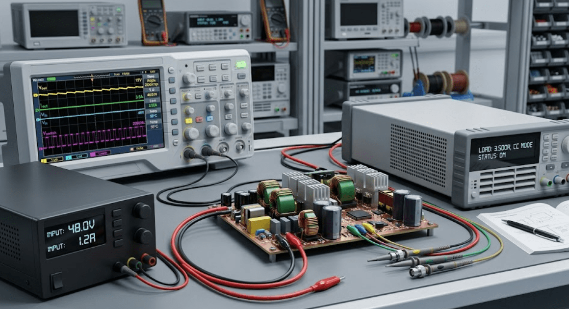
This piece explains the difference between SIL and HIL testing for power electronics, when each method fits best, and how to move between them with consistent models and test limits.
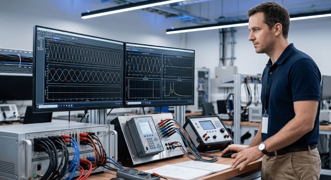
This guide explains how real-time simulation supports power system testing, how it differs from offline studies, and what model and hardware choices matter most for validation.
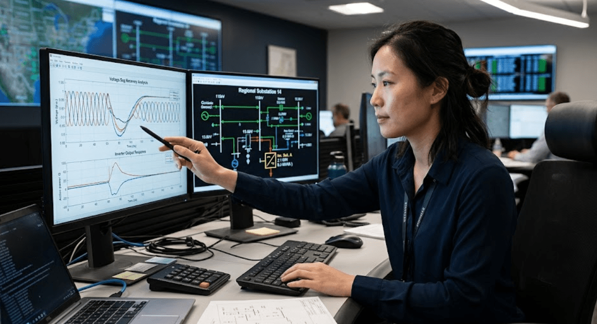
This piece explains how inverter model fidelity affects renewable grid studies, interconnection reviews, stability analysis, and IEEE 1547 compliance checks.
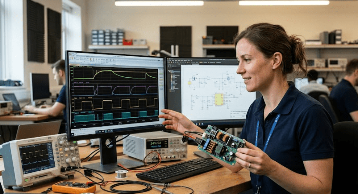
This guide explains how power electronics simulation software cuts prototype loops, where hardware still matters, and when free tools fit early design work.
A complete guide to hardware in the loop testing for power systems, covering timing, interface design, power electronics control, relay validation, software selection, and common setup errors.

This guide explains how to model an EV powertrain with clear system boundaries, suitable component fidelity, loss breakdown, regenerative braking limits, and software fit.