Key Takeaways
- Timing, limits, and signal definitions will decide if tuning results carry to hardware.
- PWM modelling depth should match loop bandwidth, with delays treated as first-class dynamics.
- Inner and outer loop separation plus worst-case stability checks will prevent late-stage surprises.
A good inverter control model will predict stability before hardware runs. You will tune faster because control stability margins stay visible. You will catch phase loss and windup early. That matters more than matching switching ripple.
Most problems start when the model is too ideal. PWM modelling that ignores update delay will overstate phase margin. Inner loop control that skips sensor filtering will overstate bandwidth. Outer loop control that assumes a fixed grid or load will break as conditions shift.
What engineers need from an inverter control model before tuning begins
Lock down what the controller sees and when it sees it before you touch a gain. Put sample time, carrier rate, delay, and measurement filtering into the model. Define every signal with units, scaling, and sign. Add limits and saturations that will exist in hardware.
A three-phase inverter switching at 10 kHz with a 50 µs step is a good test bed. Duty updates once per step, so model a one-step delay from compute to PWM output. Add the same 2 kHz current filter and sensor scaling you plan to ship. Sweep DC link from 700 V to 900 V and vary grid inductance from 0.5 mH to 2 mH.
Timing and limits decide where crossover can sit without ringing. Hidden delay steals phase and turns a safe gain into oscillation. Missing saturation hides integrator windup and makes transients look gentle. A lean model with visible assumptions will beat a detailed model with hidden ones.
“Hidden delay steals phase and turns a safe gain into oscillation.”
5 steps to build inverter control models
Follow the build order you will implement. Lock targets and limits first, then choose a PWM abstraction, then close inner and outer loops. Check stability across operating points at the end. This order stops us from tuning around modeling errors.
| Define control objectives and operating limits early | Clear numeric targets and hard limits prevent tuning gains that look stable in simulation but fail once saturation, faults, or range changes appear. |
| Select a PWM representation that matches control bandwidth | The PWM model must preserve timing and gain effects that shape phase margin, or control stability results will be misleading even if waveforms look clean. |
| Build the inner current loop with clear plant assumptions | A current loop stays predictable only when the electrical plant, sensing delay, and filtering are explicit and consistent throughout the model. |
| Add the outer voltage or power loop with proper separation | Outer loops remain stable when their bandwidth is intentionally slower than the current loop, reducing interaction and hidden instability. |
| Check control stability across operating points and delays | Stability must be verified at worst-case voltage, impedance, and delay conditions, not only at nominal operating points. |
1. Define control objectives and operating limits early
Write objectives as numbers you can test, not as intentions. Pick the regulated variable, settling time, peak deviation limit, and steady-state error. Define the operating range for DC voltage, grid or load impedance, and any derating rules. Put current, voltage, and duty limits into the model as saturations and clamps. A 5 kW inverter might target 2 ms current settling while capping phase current at 12 A peak and clamping duty if DC drops under 720 V. Add what the controller does at the limit, such as freezing the integrator, back-calculating, or rate-limiting the reference. Write one pass-fail check per objective so tests stay consistent. Clear targets stop you from tuning a waveform that looks clean but violates limits on hardware.
2. Select a PWM representation that matches control bandwidth
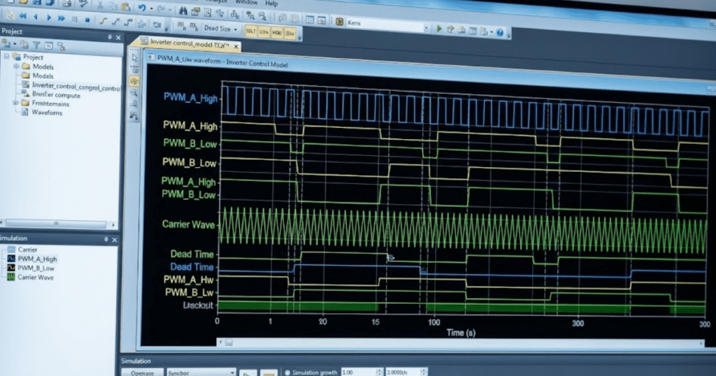
Choose a PWM representation that preserves the delay and gain your controller will see. An averaged modulator fits loop design when crossover stays well below the carrier, but it still needs a duty update delay. A sampled-data modulator matters when bandwidth approaches one tenth of switching, since sample-and-hold lag steals phase. A switching model is for ripple, harmonics, deadtime effects, and filter resonance checks. A 1 kHz current loop with a 10 kHz carrier will tune reliably on an averaged model that includes one control-step delay and the correct modulator gain. Keep a second, switching-level model in SPS SOFTWARE if you want to verify ripple without rewriting the controller. Choose the simplest model that preserves stability margins, then add detail only where results disagree.
3. Build the inner current loop with clear plant assumptions
Inner loop control starts with a plant you can explain in one line. Model the filter you have, then keep the same sign convention and reference frame everywhere. Put sensing delay and filtering inside the feedback path, not as a plotting detail. With an L filter of 2 mH and 0.15 Ω resistance, the plant is close to 1/(Ls + R) before discretization. Discretize at a 50 µs step, then tune PI gains for a crossover near 1 kHz with margin left for delay. If you use an LCL filter, keep crossover well below the resonance peak. Treat any extra filter pole as lost phase you must budget. Add anti-windup early so a current clamp does not turn recovery into a slow drift.
4. Add the outer voltage or power loop with proper separation
Outer loop control will stay stable only when it is slower than the current loop. Pick the outer objective up front, because DC-link voltage control and AC voltage control see different plants. Treat the outer plant as uncertain, since grid strength and load type will vary. Keep the outer bandwidth at least 5x to 10x lower than the current loop so interactions stay small. A DC-link loop at 20 Hz to 50 Hz feeding a 1 kHz current loop will handle load steps cleanly. A grid-forming voltage loop around 100 Hz will still sit below the current loop, but it will require clean voltage sensing. Add rate limits and windup protection so the outer loop does not keep pushing when the inner loop is saturated.
“Choose the simplest model that preserves stability margins, then add detail only where results disagree.”
5. Check control stability across operating points and delays
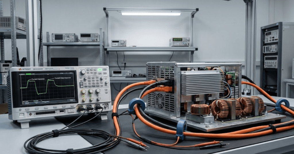
Check control stability with the full loop, not an ideal diagram. Keep sampling, PWM delay, sensing filters, and saturations inside the loop model when you assess margins. Evaluate worst cases, including minimum DC voltage, maximum power, and a weak-grid impedance point. One stress test doubles grid inductance so an LCL resonance shifts toward crossover. Another test steps current reference into the limit so you see windup and limit cycling. Use loop gain plots to catch phase loss, then confirm with a time-domain step that includes clamps. Aim for margins you can live with after discretization, such as 45° phase margin and 6 dB gain margin. Keep a short regression set so small edits do not silently shrink margins across cases.
Applying these steps to avoid unstable or misleading control results
Unstable results usually trace back to hidden timing or hidden limits. A controller tuned with zero delay will look stable and then ring once a one-step update appears. A controller tuned without saturations will look linear and then stick during faults. Tight models keep these traps visible.
Picture a loop tuned on an averaged plant at 1 kHz crossover. Add a 2 kHz sensor filter and a 50 µs compute delay and phase margin drops. Fix the timing mismatch first, then adjust gains with the same tests each time. Keep three repeatable checks, a current step, a DC sag, and an impedance sweep.
Write assumptions where everyone can see them, then keep them under version control with the model. That habit makes tuning transferable across students, researchers, and product teams. SPS SOFTWARE helps when you need component equations and controller timing exposed so reviews stay concrete. Consistent execution will keep loops calm across operating points.