Key Takeaways

• Input voltage range should set topology choice first, because a source that crosses the target output will push a simple buck or boost stage out of regulation.
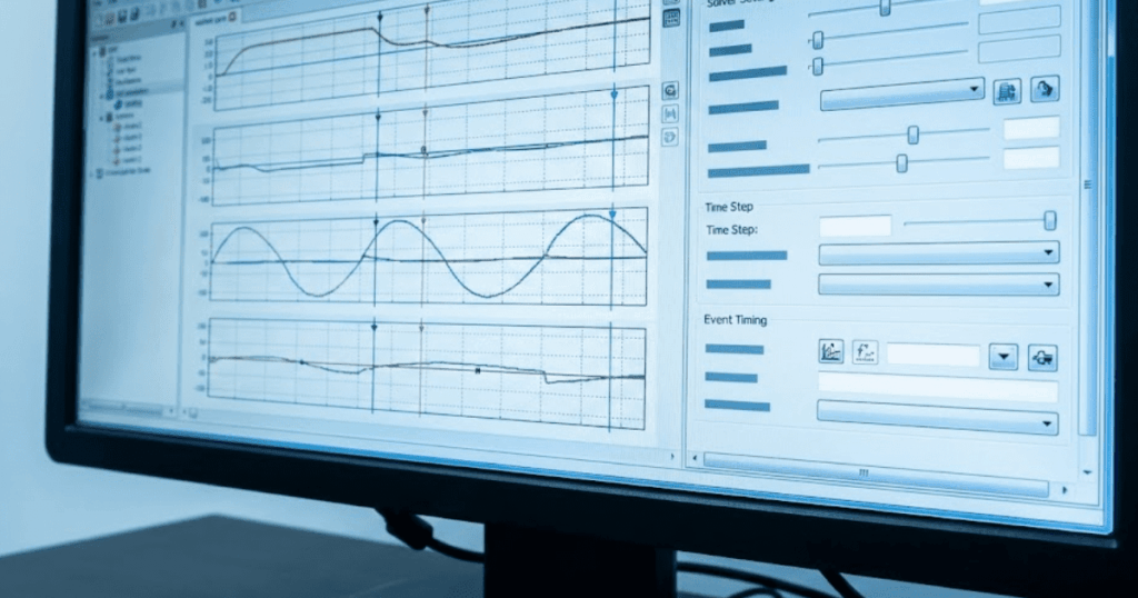
• Simulation works best when ideal switching is verified first and losses are added in steps, since that keeps the source of each waveform change visible.
• Parasitics and duty cycle limits carry more weight than clean nominal values, especially in battery-fed systems such as electric vehicle converters.

Buck boost selection starts with the input voltage range, not the converter name.

A lithium-ion cell commonly spans about 3.0 V to 4.2 V during use, which means any pack built from those cells will cross meaningful voltage limits as charge falls. That single fact separates easy converter choices from risky ones. If your source stays fully above or fully below the load target, a simple buck or boost stage will usually fit. If the source crosses the target, a buck boost converter will be the safer model to start with.

That framing matters in simulation because topology errors look acceptable until duty cycle, current ripple, and device stress are checked across the full input range. You are not choosing between three names that do the same job with small differences. You’re choosing the current path that will shape losses, control effort, and usable operating range. Good models make that visible early, before bench work turns a clean schematic into a noisy surprise.

Buck boost fits sources that cross the target voltage

A buck boost converter fits best when your input voltage will move above and below the required output during normal operation. That operating window is the main reason to choose it. It will regulate across the full span where a buck stage or a boost stage alone will lose control at one end.

A battery pack feeding a 48 V bus shows the pattern clearly. Fresh off charge, the pack might sit above 48 V, so a buck stage will work. Near depletion, the same pack can drop below 48 V, so the circuit now needs boost action. A buck boost converter covers both conditions without handing regulation from one stage to another.

This matters because many early models are built around nominal voltage only. That shortcut hides the exact operating points where duty cycle rises, current ripple worsens, and thermal stress starts climbing. If you size the converter around minimum and maximum input first, topology choice becomes much more obvious.

“If you size the converter around minimum and maximum input first, topology choice becomes much more obvious.”

Buck boost action comes from storing energy then releasing it

A buck boost converter works by storing energy in an inductor during one switch state and releasing that energy to the output during another. The control loop adjusts how long each state lasts. That timing lets the stage produce an output above or below the input, depending on circuit form and duty cycle.

A simple inverting buck boost shows the sequence well. When the switch closes, current ramps through the inductor and energy builds in its magnetic field. When the switch opens, the inductor forces current through the diode into the output capacitor and load. The average output level follows the duty ratio, so longer on time raises conversion effect.

You will see the same idea in non-inverting forms used in many power systems. The details differ, but the modelling priority stays the same. Watch inductor current, switch current, and capacitor ripple first. Those waveforms tell you more about converter health than the output voltage alone.

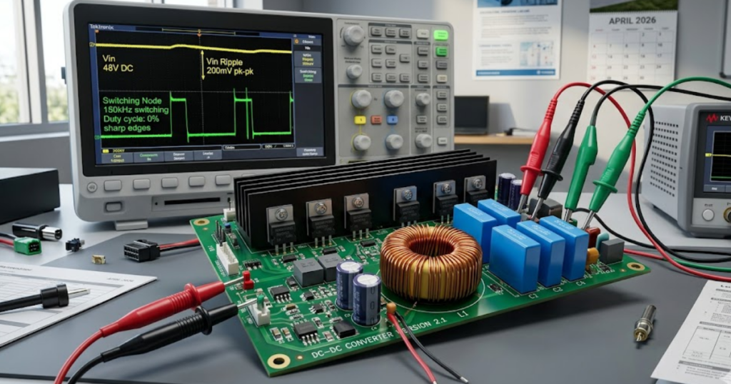
Buck stages cut voltage with simpler current paths

A buck converter lowers voltage with a simpler current path than a buck boost converter, which makes it easier to model and usually easier to control. It fits when the minimum input always stays above the target output. Source current is also more continuous, which often reduces input filtering effort.

A 24 V supply feeding a regulated 12 V controller rail is a clean buck case. The switch applies the input to the inductor for part of each cycle, and the inductor averages that pulsed energy into a lower direct current output. Output ripple is set mainly by switching frequency, inductor value, capacitor size, and parasitic resistance.

You will usually pick buck first when the voltage window allows it because fewer stressed conditions need to be checked. Duty cycle stays in a comfortable middle range more often. That usually means easier compensation, lower peak current, and fewer surprises when the model moves from ideal parts to practical ones.

Boost stages raise voltage through inductor energy transfer

A boost converter raises voltage by charging an inductor from the source and then forcing that stored energy into the load at a higher output potential. It works well when the maximum input always stays below the target output. The tradeoff is that source current and switch stress rise sharply as duty cycle approaches its upper limit.

A 12 V battery feeding a 24 V auxiliary bus is a typical boost case. The inductor charges while the switch is on, and the output capacitor supports the load during that interval. When the switch turns off, the inductor current adds to the source through the diode, which lifts the output above the source voltage.

You should treat high duty cycle results with suspicion, even when the output looks stable. Small errors in switch loss, diode drop, or inductor resistance will distort efficiency quickly. That is why boost models need a close look at current ripple and thermal rise before you accept a neat voltage trace as success.

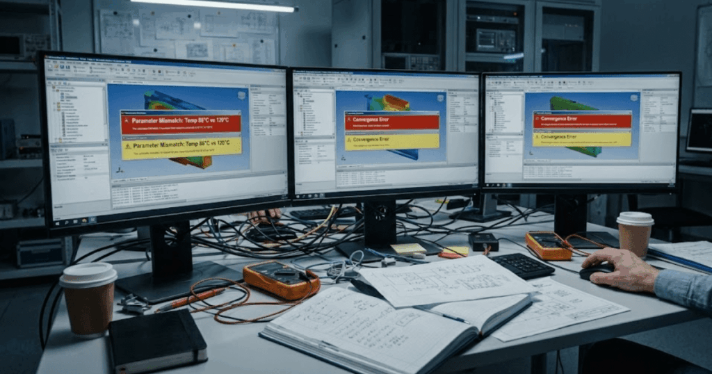
Simulation should begin with ideal switching then add losses

The best way to simulate a direct current to direct current converter is to start with an ideal switching model, verify waveforms and regulation, and then add non-ideal effects one group at a time. That order keeps faults visible. It also helps you see which parameter actually changes behaviour instead of masking several problems at once.

A useful first pass uses an ideal switch, ideal diode, nominal input sweep, and a resistive load. Once duty cycle and waveforms look correct, you add practical loss terms and compare the shift in average output, ripple, and current peaks. SPS SOFTWARE fits this workflow well because the model structure stays open enough for you to inspect each element instead of treating the converter as a sealed block.

• Start with switch timing that gives the expected output across the full input range.
• Add diode drop and switch on resistance before tuning the control loop again.
• Insert inductor winding resistance so current ripple and heating move closer to bench values.
• Include capacitor equivalent series resistance because ripple voltage will rise quickly without it.
• Model dead time and gate delay when switching loss or cross conduction matters.

That sequence will save time because each added loss has a visible signature. If output voltage collapses after resistance is added, the topology or magnetics are likely undersized. If only ripple changes, capacitor choice or frequency will need attention before control tuning starts.

Duty cycle limits explain most topology tradeoffs

Duty cycle limits explain most of the practical difference between buck, boost, and buck-boost choices. When the required duty cycle sits near 0% or 100%, current stress, loss sensitivity, and control margin all worsen. A topology that keeps duty cycle moderate across your operating window will usually produce the cleaner design.

A buck stage is comfortable when input stays well above output, because the required duty ratio stays below unity with margin. A boost stage becomes strained as output rises far above input. A buck boost stage keeps regulation across a wider span, but it pays for that range with more current stress and more parts to tune.

Buck boost suits EV batteries that cross the bus

A buck boost converter suits electric vehicle power stages when battery voltage will cross the required bus or subsystem voltage over charge state, temperature, and load. That condition appears often in traction support rails, auxiliary buses, and battery interfacing stages. The topology keeps regulation intact when a buck stage or boost stage alone would fall out of range.

An electric vehicle battery does not sit at one fixed number during use, and that is why this topology matters. Global battery electric car sales reached about 14 million in 2023, equal to roughly 18% of all car sales. A wide and growing installed base means more engineers are modelling battery-fed converters across full operating windows rather than around nominal pack values.

A practical case is a high-voltage pack feeding a lower auxiliary rail during one mode and accepting power from a lower source during another. The exact control scheme will vary, but your model should always sweep minimum pack voltage, maximum pack voltage, and step load conditions. That is where converter choice stops being academic and starts showing its fit.

“Good converter selection comes from that discipline, because the right stage is the one that keeps its behaviour when the ideal parts are gone.”

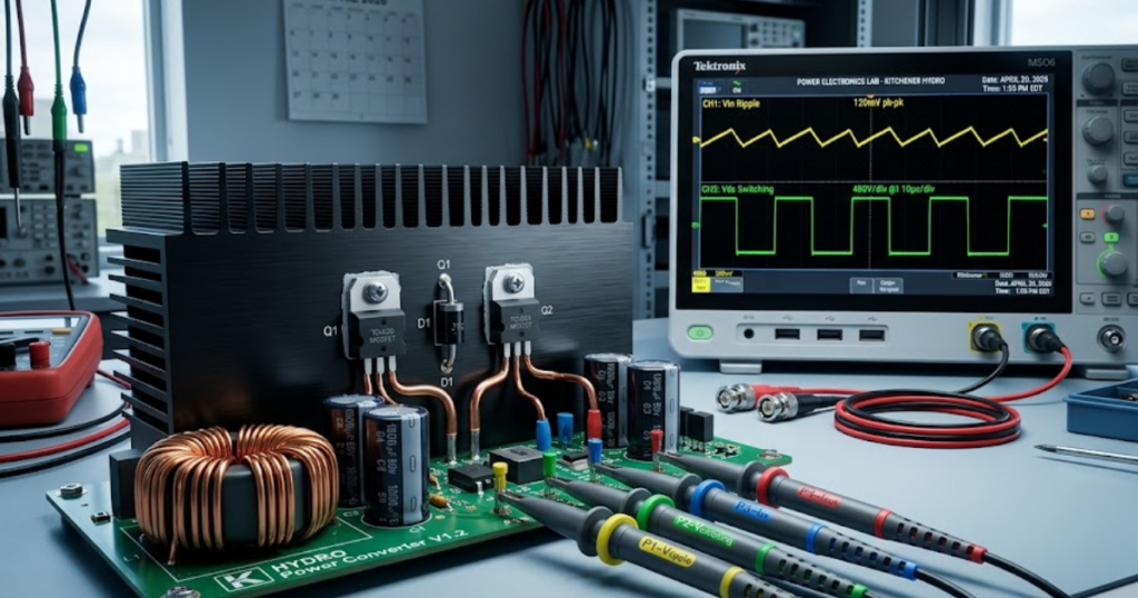
Parasitics decide if simulated gains survive hardware build

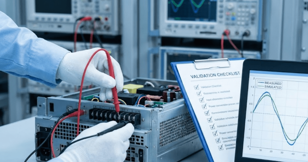
Parasitics decide whether a converter that looks strong in simulation will still behave once copper resistance, capacitor loss, layout inductance, and device timing enter the picture. These effects are not small corrections. They will reshape ripple, peak current, voltage overshoot, and efficiency enough to overturn an early topology choice.

A bench build often exposes this gap at the switching node. The ideal model shows clean transitions, while the hardware shows ringing, extra heating, and output ripple that seemed absent before. That usually traces back to ignored equivalent series resistance, loop inductance, or recovery behaviour. Once those terms are present, the best topology is the one that still meets the target with margin rather than the one that looked best on a clean schematic.

That is the useful habit to keep after the first successful run. SPS SOFTWARE works best when you treat every component as inspectable and editable, then tighten the model until it explains the waveform you expect to measure. Good converter selection comes from that discipline, because the right stage is the one that keeps its behaviour when the ideal parts are gone.

Key Takeaways

• Voltage stability analysis works best when you track reactive power margin, equipment limits, and control saturation instead of relying on voltage magnitude alone.
• PV curves, QV studies, and dynamic simulation answer different questions, so the right study sequence will save time and improve the quality of your engineering judgment.
• Protection coordination, feeder load behaviour, and inverter current limits will decide whether simulated margin is credible enough to support operating or planning choices.

Voltage stability analysis in simulation works when you treat reactive power margin as the main signal, not voltage magnitude alone.

Voltage collapse rarely starts as a single low-voltage reading. It starts when generators, capacitor banks, static compensators, or inverter controls run out of reactive support while transfer stress keeps rising. Wind and solar produced 13.4% of global electricity in 2023, which means more grids now depend on converter behaviour that must be represented properly in stability studies. Good voltage stability analysis will show you where the weak buses are, which limits bind first, and how protection will react when voltage recovery slows.

Useful simulation comes from disciplined model choices, not from a single study type. You’re trying to answer a practical engineering question about margin, collapse risk, or corrective action. That means your model will need credible load behaviour, realistic control limits, and a study method matched to the disturbance or loading pattern you care about. If those pieces are wrong, the plots will look clean and still tell you the wrong story.

“The key measure is reactive power margin.”

Voltage stability is about reactive power margin

Voltage stability is the ability of a power system to maintain acceptable voltage after load growth, switching, or a disturbance. The key measure is reactive power margin. A bus can sit near nominal voltage and still be close to collapse. That is why voltage magnitude alone won’t tell you enough.

Consider a transmission corridor feeding a heavy urban load pocket on a hot evening. Tap changers keep distribution voltage near target, induction motors draw more reactive current, and a nearby generator reaches its reactive limit. The voltage profile can still look acceptable for a short period, yet the system has almost no extra support left. A small line outage or another step in loading will push the bus toward the nose of the power-voltage curve.

This matters because voltage instability is usually a limit problem before it becomes a visible low-voltage problem. You need to track generator reactive ceilings, switched compensation steps, transformer tap action, and load sensitivity to voltage. If you don’t, you’ll confuse a healthy operating point with a fragile one. Good analysis starts with the question, “How much support is left before controls saturate?”

Start simulation with a credible network model

A credible network model includes the parameters and controls that actually shape voltage response under stress. You need correct line data, transformer taps, shunt devices, generator limits, load composition, and control logic. If any of those are simplified too far, the margin you calculate won’t match field behaviour.

A practical setup begins with a solved base case and a clear study boundary. A feeder study needs feeder regulators, capacitor switching logic, and motor-rich loads. A bulk system study needs generator excitation, reactive capability limits, and transfer paths that reflect the operating condition you’re testing. In SPS SOFTWARE, that execution step is useful because you can inspect and edit model equations and protection settings instead of accepting a closed result.

The fastest way to lose confidence in voltage stability analysis is to skip basic model checks. Use this minimum checklist before you start stressing the system.

• Confirm the base case power flow matches the intended operating condition.
• Check every reactive source for realistic limits and control priorities.
• Represent loads with voltage sensitivity that fits the study area.
• Verify transformer tap ranges, deadbands, and time delays.
• Include protection elements that will trip before collapse is complete.

Use PV curves to locate weak buses first

PV curve analysis is the quickest way to find where voltage stability margin is thin. You increase loading or transfer stress step by step and watch how bus voltage responds. The weak buses are the ones that approach the nose first. Those buses deserve your attention before deeper studies begin.

A common workflow stresses a transfer corridor from a generation area into a load area while monitoring several buses. One bus will usually show a sharper voltage drop and a smaller loadability margin than the others. That bus becomes the anchor point for corrective action screening. You can then test shunt support, generator redispatch, or tap adjustments and see which measure shifts the nose to a safer operating point.

PV curves are valuable because they turn a vague concern about collapse into a ranked map of weak locations. They also keep you from spreading effort across the whole network when the limiting problem is local. You’ll get the most value when each step respects equipment limits and control actions. If reactive ceilings are ignored, the curve will look better than the system really is.

Use QV studies when reactive limits dominate

QV studies answer a narrower but very important question. They show how much reactive injection a bus needs to maintain a chosen voltage level. That makes them useful when the main issue is local support deficiency. They are less about loadability and more about reactive deficiency at a specific location.

A weak substation bus near a large motor load is a good case. The PV curve can confirm that the area has poor margin, but the QV curve will show how much reactive support is required to hold 1.0 per unit or another target. That makes capacitor sizing, static compensation studies, and support placement more concrete. You’re no longer guessing which bus needs help or how much help it needs.

QV results become especially important after generator reactive limits are reached or after a line outage changes local VAR supply. They also expose cases where a bus needs support that a distant source can’t deliver effectively because of transmission reactance. If your question is “Where do I place support and how much is required?” a QV study will answer it more directly than a PV curve.

Dynamic simulation tests the path toward voltage collapse

Dynamic simulation shows how the system moves from a disturbance toward recovery or collapse over time. It captures control action, delay, saturation, and protection logic that static studies cannot represent fully. That is why it is essential after PV and QV studies identify weak areas. Static margin tells you the distance to trouble, while dynamic response shows the route.

A bus fault cleared after several cycles can leave motors stalled, transformer taps moving, and reactive devices switching in sequence. A static study will miss that timing. An RMS model can show slow voltage recovery after fault clearing, and a more detailed electromagnetic model can show converter current limiting or control interaction during the same event. Those details matter when the operating point is already close to its reactive ceiling.

Use this checkpoint to match the study method to the question you’re asking.

Distribution networks need load models that match behaviour

Distribution voltage stability studies will fail if load models are too simple. Feeders are shaped by motors, thermostatic loads, rooftop generation, regulator action, and unbalance. Constant power assumptions can overstate or understate collapse risk. You need behaviour that matches the actual feeder mix.

A long feeder serving air conditioning, small commercial motors, and distributed generation will respond very differently from a feeder made mostly of resistive heating. After a fault or voltage dip, motor stalling can hold reactive consumption high while regulators and capacitor controls respond with delay. If your model treats all of that as a static constant power block, the predicted recovery will look smoother than the feeder will actually deliver.

Distribution studies also need attention to where controls act and how quickly they act. Tap changers can support customer voltage while pushing the upstream system closer to its limit. Capacitor banks can help one section and worsen another if switching logic is poorly timed. You can’t study voltage collapse risk on a feeder as if it were a reduced bulk bus. The feeder’s composition is the study.

Grids with high renewable share need inverter limits

Renewable-heavy grids need explicit inverter current limits, control priorities, and reactive support settings in the model. Converter-based resources do not respond like synchronous machines. When voltage drops, their controls will follow current limits and protection thresholds. If those limits are missing, the simulated margin will be overstated.

A solar plant tied to a weak grid offers a clear case. During a voltage dip, the inverter controller will often prioritise reactive current support up to a current ceiling. Past that ceiling, active power support falls and further voltage support is capped. Solar photovoltaic generation rose by almost 320 TWh in 2023, the largest annual increase ever recorded, which makes this modelling detail important for modern stability studies.

You’ll also need to represent plant-level voltage control, collector system impedance, and grid code settings that govern fault ride-through. A generic source behind a reactance won’t capture those limits. That shortcut might be acceptable for rough screening, but it won’t support a credible judgment about collapse risk. If your network is rich in inverter-based resources, the voltage stability model has to reflect converter physics and control logic.

“A margin that exists only before a relay trip is not usable margin.”

Protection coordination must reflect voltage stability limits

Power system protection coordination is part of voltage stability analysis because protection will define the final outcome once voltage recovery slows or current rises. A margin that exists only before a relay trip is not usable margin. You need the study to reflect the same trip logic the field equipment will enforce.

A delayed undervoltage trip on a wind plant, a load-shedding stage on a weak feeder, or an overexcitation limiter on a generator can each alter the path from disturbance to collapse. One setting can preserve service long enough for voltage recovery, while another can remove support and deepen the dip. That is why protection review belongs inside the simulation workflow instead of after it. If the relay clears first, your PV or QV result won’t be the whole answer.

The best engineering judgment comes from lining up margins, control limits, and protection timing in one consistent model. SPS SOFTWARE fits naturally in that workflow because open models make it easier to inspect the assumptions behind network response and relay action. You’re not looking for a dramatic plot. You’re looking for a study result that still makes sense when the system is stressed, the controls saturate, and the protection acts exactly as set.

Key Takeaways

• Reproducible EMT research starts when you treat the simulation run as a complete, rerunnable record that includes the model, numerics, inputs, and tool versions.
• Physics-based model transparency matters as much as results, because readers need to inspect equations, assumptions, and control logic to trust that the same study is being rerun.
• Most repeatability failures come from small, undocumented choices such as time step, event timing, initialization, and post-processing, so disciplined run manifests and portable study packaging should be standard practice.

Reproducible simulation research fails most often when authors treat a simulator run as a screenshot instead of a record you can rerun. A large survey found 70% of researchers had tried and failed to reproduce another scientist’s experiments. EMT research carries extra risk because small numerical and modelling choices can shift waveforms, trip logic, and protection outcomes.

“You can make EMT power system results repeatable when you publish the model, the numerics, and the run conditions as a single package.”

The practical stance is simple: reproducibility is a design requirement for your study, not a clean-up task after you’ve written results. Physics-based modelling makes that achievable because equations, parameters, and assumptions can be inspected and challenged. Your job is to keep every hidden decision visible, from solver tolerances to initial conditions, so a reviewer or lab partner can rerun the study and reach the same technical conclusions.

Define reproducible simulation research in EMT power system studies

Reproducible EMT research means an independent reader can run your simulation model and obtain the same key plots and metrics within a stated tolerance. It includes the full model, all inputs, and the numerical settings used to generate results. It also includes tool versions and any external scripts. It is stricter than claiming similar behaviour.

For EMT work, “same result” should be defined in engineering terms, not aesthetics. If your claim depends on peak current, DC link ripple, PLL stability, or protection pickup time, you need a numeric acceptance band for those outputs. That band should reflect numerical noise you expect from different machines, not the spread you get from undocumented parameter choices.

It also helps to separate three levels of repeatability so your readers know what to expect. Repeatable runs on the same computer test basic run control. Reproducing on a different computer tests tool versioning, floating point differences, and hidden dependencies. Reproducing in another simulator tests modelling assumptions, and that requires even clearer documentation of physics-based equations and control logic.

Specify model transparency requirements for physics-based power system modelling

Transparent physics-based models expose equations, parameters, and component limits so others can inspect what your study actually simulates. You should be able to trace any plotted waveform back to a component model and a parameter value. Control blocks must be readable, not compiled into opaque artefacts. If a value is tuned, the tuning target must be stated.

Start with a tight “model contract” that defines what is inside the scope and what is not. If you use an averaged converter model, state the switching details you removed and why that is acceptable for your claim. If you include detailed switching, state how you represent device losses, dead time, and saturation. Readers do not need every intermediate note, but they do need every assumption that changes physics.

Transparency also includes naming and structure. Consistent signal names, clear subsystem boundaries, and readable units reduce the risk that another researcher wires something incorrectly and blames the tool. When a model is clear enough for a graduate student to audit, it is usually clear enough for a reviewer to trust.

Control numerical settings that most often break reproducibility

EMT reproducibility breaks when solver choices, time step, interpolation, and event handling are treated as defaults. Time step and tolerances directly affect switching ripple, control stability margins, and protection timing. Event timing rules, such as breaker operation and fault insertion, must be specified precisely. You should publish these settings as part of the study definition, not as simulator trivia.

Consider a grid fault study on a 2 MW inverter model where your claim depends on the first 10 ms of current limiting. A fixed time step of 5 µs can show a different peak and a different limiter activation instant than 20 µs, even with identical controller gains, because sampling, discretization, and switch event alignment shift. If the paper reports only the controller diagram and omits the numerical settings, another lab can “replicate” the model and still miss your headline result.

Set explicit rules for how you choose numerics. Start with a time step justified by the fastest dynamics you keep, then confirm key outputs are stable under a smaller step. State any filters or decimation used for plots so readers do not confuse display smoothing with physical damping. When your results depend on threshold crossings, record the detection method and the comparison tolerance.

Record inputs, initial conditions, and solver versions consistently

Repeatable EMT studies require a complete run record that captures every input, initial state, and tool version used. Initial conditions matter because controls, machine states, and network voltages can settle into different trajectories. Versioning matters because solvers, libraries, and numerical fixes change behaviour. If you can’t recreate your own figures six months later, nobody else will.

Use a run manifest that travels with the model and gets updated every time you regenerate results. Treat it like a lab notebook entry with strict fields, not free text. When you work with teams, a manifest becomes the shared reference that prevents quiet drift between “the model” and “the results.”

• Simulation tool name, exact version, and operating system details
• Solver type, fixed or variable step, time step, and error tolerances
• All input files with checksums and a single source of parameter values
• Initial condition method, including any power flow or steady-state pre-run
• Event schedule with timestamps for faults, switching, and controller mode changes

The same discipline applies to scripts used for plotting and post-processing. If a plot uses windowing, resampling, or filtering, record the settings and the code version. A clean run record turns review comments into quick reruns instead of weeks of reconstruction.

Package and share EMT studies so others can rerun

“Sharing for reproducibility means shipping a runnable bundle, not a diagram and a parameter table.”

A complete package includes model files, the run manifest, input datasets, and the plotting scripts that generate published figures. File paths must be relative and portable so the project opens on a new machine without manual repair. Your goal is a single command or click that reproduces the outputs you cite.

Packaging works best when you separate editable source from generated artefacts. Keep source models, parameter sets, and scripts under version control, and store generated plots in a results folder tied to a specific commit. Archive the exact run bundle associated with a submission so later edits do not overwrite the provenance of published figures.

Some teams standardize this workflow inside SPS SOFTWARE because open, editable component models and clear parameterization make it easier to bundle what matters for reruns. The tool choice matters less than the habit: if the recipient cannot inspect and execute what you used, the study cannot be reproduced.

Detect common reporting gaps that block repeatable results

The fastest way to improve reproducibility is to look for gaps reviewers repeatedly hit: missing numerics, missing initial conditions, and missing event definitions. These omissions are not minor, because EMT outputs can shift with tiny differences. A separate survey finding showed 52% of researchers agree there is a significant reproducibility crisis. That pattern matches what power system reviewers see when simulation results can’t be rerun.

A simple self-test catches most issues before submission. Another person on your team should be able to clone the study bundle, run it on a clean machine, and regenerate every figure without asking you questions. If they need an email thread to find solver settings, a parameter file, or the exact event timing, the paper is not ready for scrutiny.

Good reproducibility feels strict, but it pays off in calmer review cycles and cleaner internal handoffs. Teams that treat modelling as a publishable artifact, not a personal workspace, build credibility that accumulates over time. SPS SOFTWARE fits best when you want that discipline supported by transparent, inspectable physics-based models, yet the outcome still depends on your run records and packaging habits.