Key Takeaways
- Large SPS Software models only become useful for real-time work when structure, solver settings, and data handling are tuned with the same care as the electrical design itself.
- Simplifying hierarchy, selecting the right solver strategy, and replacing non-essential detailed components with reduced models can cut run times significantly without sacrificing the physics that matter.
- Profiling is a practical way to see where simulations actually spend time, which helps you focus optimization on specific subsystems, control loops, and logging choices that have the biggest impact.
- Careful management of sampling rates, timing margins, and memory usage improves both numerical accuracy and throughput, so you can run more scenarios and gain clearer insight from each one.
- SPS Software provides an integrated workflow for MATLAB model optimization, helping engineers, educators, and researchers move large simulation models from offline analysis to real-time targets with confidence.
Every engineer who has watched a progress bar crawl during a long simulation knows how painful a slow model feels. Large SPS Software models can be rich in detail, yet that complexity often causes missed real-time deadlines and stalled work. You might have controllers waiting on signals, processors pegged at full utilisation, and hardware-in-the-loop setups that simply cannot keep up. Tuning those large simulation models for speed and robustness turns frustration into predictable timing, cleaner results, and calmer test days.
Power systems engineers, power electronics specialists, grid planners, and researchers all feel this pressure when models grow beyond a few thousand states. You need accurate physics-based behaviour for feeders, converters, or microgrids, yet you also need simulations that finish before the lab closes. That balance becomes even more sensitive once SPS Software models feed hardware platforms for hardware-in-the-loop or real-time validation. Teams in academia and industry face offline queues, limited real-time access, and higher expectations for system studies, which puts extra weight on every modelling choice.
“Tuning those large simulation models for speed and robustness turns frustration into predictable timing, cleaner results, and calmer test days.”
Why optimizing large-scale SPS Software models is critical for real-time performance
Large-scale SPS Software models often start life as exploratory studies, with high detail everywhere and little thought given to solver cost. That structure works for overnight runs on a workstation, but the same model typically exceeds the time budget once you target a real-time processor. Every extra state, discontinuity, and algebraic loop adds work for the solver, and that effort shows up as missed step deadlines and jitter. During hardware-in-the-loop work, those overruns can stop tests, upset controllers, or hide faults that only appear when timing is correct. Optimizing large simulation models at this stage means shaping them so each time step finishes within the real-time window, while still reflecting the physics you care about.
Real-time performance is not just about raw speed, because accuracy suffers if the solver cuts corners to stay on schedule. Faster models let you sweep more scenarios, stress controllers over longer time spans, and test rare edge cases that might never show up in a single long run. Once results match across offline and real-time runs, you gain confidence that any failure you see comes from the design, not from numerical artefacts or overloaded processors. This combination of timing reliability and trustworthy waveforms is what turns SPS Software optimization from a pure performance exercise into a foundation for better engineering judgement.
5 optimization tips for large-scale SPS Software models
Effective SPS Software optimization starts with a clear view of where simulation time actually goes. Some of that cost comes from how you structure the model, and some comes from solver settings or data handling choices. Small structural changes in SPS, especially for large simulation models, often yield bigger gains than switching hardware or adding processing cores. Optimisation work that targets structure, solvers, components, profiling, and data handling usually fits directly into the way you already build and test models.
1. Simplify model hierarchy to reduce solver load
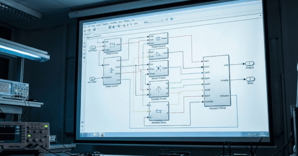
Complex hierarchy is often the first hidden source of cost in SPS models built on top of MATLAB and Simulink diagrams. Deep nesting of subsystems, conditional subsystems, and masked components forces the engine to manage many execution contexts, even when electrical behaviour remains simple. Bringing related blocks into flatter, well-grouped sections reduces that overhead and makes execution order easier to reason about. You still keep logical separation for teaching or documentation, while the solver sees fewer layers to walk through at each step. Many teams create a clean top level dedicated to power system structure, then push only essential reusable logic into subsystems with clear naming and minimal nesting.
Large grid or converter studies often include repeated feeders, load banks, or converter legs that share the same structure but differ in parameters. Creating parameterised subsystems for these patterns gives you one place to tune structures while avoiding extra depth from excessive grouping. You can also remove layers that only serve visual layout, such as subsystems used purely to box blocks on the screen, replacing them with annotations or area highlights. This type of clean up helps students and junior engineers read the model faster, which reduces modelling errors that later show up as unstable real-time runs. Structured hierarchy that stays shallow but clear becomes easier to port to hardware targets and to share across academic or industrial teams.
2. Use variable-step solvers efficiently for faster simulation
Variable-step solvers help accelerate offline SPS runs by adapting the time step when signals change slowly, yet they still require careful configuration. Loose error tolerances, stiff systems, or many fast switching elements can cause step chopping that undermines performance gains. Start from recommended solver settings for your mix of electrical and control components, then tighten tolerances only where they affect results that matter for your study. Engineers often see major MATLAB model optimization wins simply by measuring step sizes over time and avoiding extreme fluctuations that indicate solver stress. Once the offline model behaves well, you can switch to an equivalent fixed-step configuration for real-time work with fewer surprises.
For large simulation models that mix slow electromechanical dynamics with fast switching or protection logic, consider partitioning components across multiple solver rates. Slow states such as mechanical shaft dynamics or averaged grid equivalents can use longer effective steps, while switching and protection elements run on shorter steps only where needed. This type of multi-rate strategy reduces the number of tiny integration steps that otherwise propagate across the entire system. You can then validate accuracy with time-domain overlays, frequency-domain comparisons, or power balance checks to ensure that solver tuning has not hidden important behaviour. Iterating in this structured way keeps solver choice aligned with physics rather than chasing trial-and-error settings.
3. Replace detailed components with equivalent simplified subsystems
High fidelity component models feel comforting, yet full switching models for every converter leg or detailed network for every feeder quickly overload real-time targets. Averaged models, Thévenin equivalents, or reduced-order machines often capture the behaviour you need while cutting states and discontinuities dramatically. For example, a cluster of photovoltaic inverters feeding a common bus can share a single averaged interface plus a smaller set of detailed models used only where switching artefacts matter. When models support teaching, you can preserve detailed views in separate subsystems and offer simplified equivalents as the default for performance. Students still learn how the full circuit behaves, while lab sessions remain practical on shared real-time hardware.
Simplification works best when guided by clear questions about what outputs matter and which inputs drive those outputs most strongly. If your objective is to validate controller behaviour for fault scenarios, the model must preserve fault timing, voltage and current envelopes, and any nonlinearities that influence controller decisions. Fine detail in remote parts of the network or secondary subsystems often contributes little to those quantities and can move into simpler equivalents. Documenting these choices directly in the model, for example through annotations or variant controls, helps future users understand the limits of each configuration. Clear justification for each simplified subsystem also reassures reviewers and project sponsors that performance gains do not hide important physics.
4. Profile model execution to identify computational bottlenecks
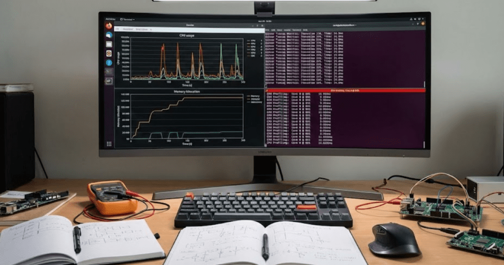
Profiling tools in MATLAB and Simulink give a concrete view of where simulation time is spent for SPS models. Instead of guessing which part of a large diagram is slow, you see exact functions, subsystems, and blocks that consume the most steps or CPU cycles. Engineers often discover that a few oscillating control loops, high-frequency measurement filters, or diagnostic scopes account for a large share of runtime. Removing unnecessary logging, simplifying control logic, or retuning filters in those locations typically delivers bigger gains than blanket changes to the entire model. Profiling also reveals parts of the model that never execute during a given scenario, which may signal dead code, unused protection paths, or features that should move into separate test cases.
Real-time preparation benefits from profiling across multiple test cases, such as normal operation, faults, and start-up sequences. Some bottlenecks only appear during limit cycles or edge scenarios, so it helps to profile those paths before deploying to hardware. You can store profiler results alongside the model, which lets team members review past decisions on solver choices and subsystem restructuring. This shared context prevents repeated tuning work and builds confidence that optimizations are based on measured data rather than intuition alone. Profiling becomes part of the modelling culture, much like unit testing for software, which improves quality across projects over time.
5. Pre-allocate data and manage signal logging for memory efficiency
Memory usage often limits large SPS models before pure computation does, especially when many signals log to the workspace or external files. Logging every waveform at full resolution for long scenarios creates enormous datasets that slow down both simulation and post-processing. You can usually keep only key currents, voltages, and controller states at full rate, while decimating secondary signals or logging them only around specific events. Model-based logging controls, signal groups, and conditional scopes make it easy to switch between lightweight debug configurations and richer traces used for detailed studies. Keeping memory footprints modest reduces the risk of overruns on real-time targets and shortens the delay between test runs in the lab.
Pre-allocating arrays in MATLAB functions or scripts connected to your SPS models avoids costly memory growth during simulation. Growing variables one sample at a time inside control logic or data logging callbacks forces the engine to request new memory repeatedly. You can estimate required sizes from expected simulation length and sample times, then allocate once and reuse buffers across cases. This approach keeps memory access patterns predictable and helps real-time schedulers maintain consistent performance. Clean memory management pairs well with good logging practice to support longer, more informative test campaigns without frequent resets or manual cleanup.
Consistent SPS Software optimization across hierarchy, solvers, components, profiling, and data handling turns large models into reliable tools rather than fragile experiments. Each improvement may appear small in isolation, yet taken across an entire project they often cut simulation time by factors, not just percentages. Shorter, more stable runs free scarce real-time hardware for more users, more scenarios, and more ambitious studies. That improvement in throughput and confidence pays off in smoother lab schedules, clearer teaching sessions, and stronger validation for industrial projects.
“Consistent SPS Software optimization across hierarchy, solvers, components, profiling, and data handling turns large models into reliable tools rather than fragile experiments.”
How optimization improves accuracy and simulation throughput in real-time systems
Model optimisation work often starts with performance targets, yet it has direct consequences for accuracy as well. Poorly tuned solvers, inconsistent sampling, or overloaded tasks can distort waveforms even when a run appears to finish on time. Careful SPS Software optimization keeps numerical error, latency, and jitter within known limits, so that comparisons between offline and real-time runs remain meaningful. The benefits show up in several concrete ways for engineers, students, and researchers working with real-time targets.
- Higher numerical fidelity: Tight control of solver settings reduces integration error, so voltage and current traces stay closer to analytical expectations. This fidelity makes it easier to spot small controller issues, such as marginal stability or subtle overshoot, before hardware testing.
- More consistent timing: Optimised models meet step deadlines with margin, which keeps sampling instants aligned with controller assumptions. Consistent timing avoids artificial oscillations introduced purely by jitter, so faults and events occur when you expect them to.
- Greater scenario coverage per day: Faster simulations let you run more load levels, fault cases, and parameter sweeps within the same lab slot. Higher throughput translates into better statistics and stronger confidence when presenting results to peers, managers, or examiners.
- Easier comparison between offline and real-time runs: When both versions of the model behave similarly, you can use offline studies to narrow down parameter ranges before moving to hardware. This alignment saves time on setup, reduces debugging effort, and clarifies which differences truly come from the target hardware.
- Improved hardware utilisation: Efficient models make better use of limited real-time processors and chassis, so teams can share platforms without long waiting lists. Engineers spend more hours testing designs and fewer hours waiting for a free slot, which improves learning and project progress.
- Clearer teaching and training outcomes: Students working with responsive models see the link between theory and waveforms within a single lab session. That immediacy helps concepts stick, encourages experimentation with settings, and builds confidence for future industrial projects.
Optimisation that improves both accuracy and throughput directly supports better engineering understanding and safer decision paths. You spend more time interpreting clear results and less time questioning solver behaviour or re-running unstable cases. Teams that measure these gains often find that simulation becomes a trusted part of design and validation, not just a preliminary check before experiments. Over time, well-optimised SPS workflows create a shared language of waveforms, timing margins, and performance targets that links classrooms, research labs, and industrial projects.
How SPS Software supports engineers in optimizing models

SPS Software gives modelling teams a familiar MATLAB and Simulink workflow with power-focused libraries that already reflect how electrical engineers think about systems. Open, physics-based component models let you inspect equations, adapt parameters for local grids or converters, and teach students exactly what each block computes. Because SPS Software integrates cleanly with model-based design flows, you can use the same diagrams for offline studies, automated parameter sweeps, and preparation for real-time targets. That continuity reduces rework and gives both professors and engineers a single modelling language to share across courses, research projects, and applied studies. When models scale toward real-time, SPS users can draw on established workflows for hierarchy management, solver tuning, and profiling that align with the optimization steps described earlier.
Engineers working with OPAL-RT hardware often pair SPS Software models with dedicated real-time solvers, so optimization work in SPS maps directly to gains on the target simulator. Academic labs can share example models, courseware, and profiling templates across institutions, strengthening teaching while keeping local setups affordable. Industrial teams benefit from the same transparency when they transfer models from feasibility studies into hardware-in-the-loop rigs, since every simplification or solver tweak remains visible and reviewable. This combination of open models, consistent workflows, and clear optimization practices positions SPS Software as a dependable companion for engineers who care about both understanding and performance. Teams can trust that time invested in tuning SPS models supports better teaching, more credible research, and safer industrial decisions year after year.

