
Key Takeaways
-
- Power hardware in the loop is useful when electrical interaction, not software logic, is the main project risk.
-
- Controller HIL and PHIL answer different questions, and moving up too early or too late wastes effort.
-
- Stable interfaces and disciplined model preparation decide if PHIL results can be trusted.
Power hardware-in-the-loop testing earns its place when control code looks stable in simulation but the power stage can still fail at the interface with the grid.
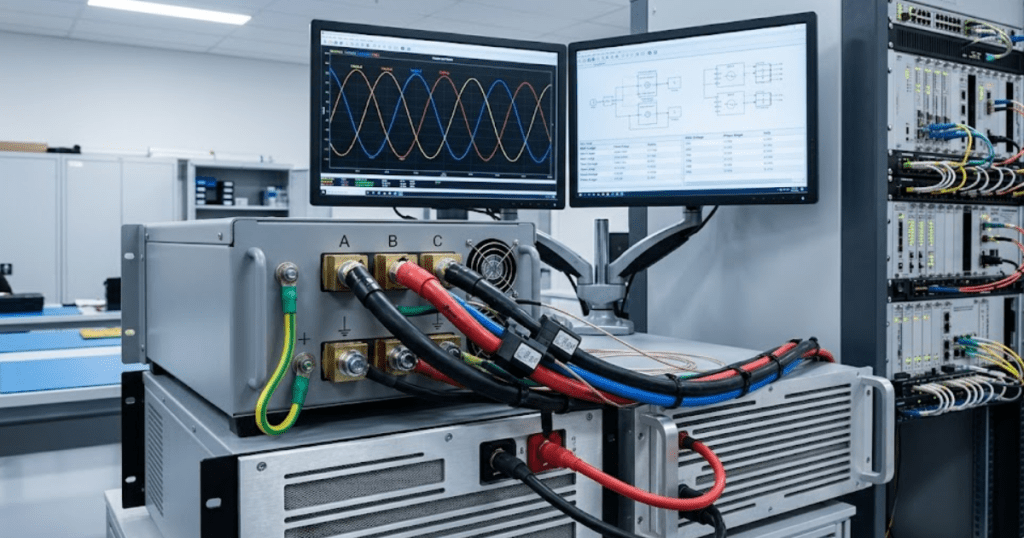
Power hardware in the loop connects a digital power-system model to physical equipment through a power amplifier, so you can test an inverter, converter, charger, or protection device under stressful electrical conditions without building the full network. Global renewable capacity additions reached almost 510 GW in 2023, and solar photovoltaic supplied roughly three-quarters of that growth. That shift matters because inverter-based equipment now meets feeders, fault events, and protection schemes under a much wider set of operating conditions.
Power hardware in the loop couples hardware to simulation
Power hardware-in-the-loop testing links a physical device under test to a simulated electrical network, then exchanges measured voltage and current through a power interface so both sides affect each other. You are no longer checking code alone. You are checking how hardware behaves when the electrical system pushes back under load.
A common setup places an inverter on the bench, keeps the grid, feeder impedance, and fault conditions in the simulator, and uses sensors plus a power amplifier to close the loop. The inverter sees voltage commands from the simulated grid, while the simulator receives measured current from the inverter terminals. That closed loop is what gives PHIL its value for power electronics and grid studies.
The important point is physical energy exchange. Once current limits, filter resonance, dead time, sensor scaling, and switching-side delays enter the loop, behaviour can depart from offline simulation quickly. That is why power hardware in the loop sits between pure software study and full prototype deployment. It lets you test electrical interaction without building the entire plant first.
Controller HIL stops short of full power interaction
The main difference between controller HIL and power hardware-in-the-loop testing is simple: controller HIL exchanges low-power signals with a controller, while PHIL exchanges actual electrical power with hardware. Controller HIL proves control logic against a simulated plant. PHIL proves the hardware and the plant interface at the same time.
“The next useful step is to expose the physical unit to the electrical conditions that will decide acceptance.”
| Checkpoint | Controller HIL meaning | Power hardware in the loop meaning |
| The interface across the bench | Signals stay at low voltage and low current between simulator and controller. | Voltage and current pass through a power amplifier to the device under test. |
| The item being validated | The focus stays on firmware, logic, scheduling, and control state handling. | The focus includes magnets, semiconductors, filters, sensors, and protection hardware. |
| The main failure it reveals | It exposes bad control logic, timing faults, and incorrect state transitions. | It exposes unstable electrical interaction, saturation, and hardware-side limits. |
| The bench cost and complexity | The setup stays lighter because no power interface is required. | The setup is heavier because amplification, sensing, and loop stability matter. |
| The reason teams move up a level | They need more confidence after software logic looks correct. | They need proof that the physical unit behaves correctly under power stress. |
A controller HIL bench can show that a current controller tracks a reference correctly, yet it cannot prove how an LCL filter, sensor noise, contactor timing, or DC-link sag will affect the physical unit. That gap is exactly where PHIL belongs. You use controller HIL first for control confidence, then move to PHIL when electrical interaction becomes the main unknown.
Use PHIL when power behaviour shapes system risk
You should use PHIL when the main project risk sits in the power path, not just in the control path. That includes projects where hardware limits, grid strength, fault response, or protection interaction will decide if the design is acceptable. If the electrical interface can make or break the result, simulation alone won’t settle it.
Clear triggers usually appear before the bench is built. A grid-following inverter aimed at a weak feeder, a battery converter with strict current limiting, or a charger that must ride through voltage dips all fit this pattern. Those cases share one theme: the plant model and the hardware must influence each other under load.
-
- Your device must exchange meaningful power with a simulated grid or feeder.
-
- Your acceptance criteria depend on current limits, voltage quality, or protection timing.
-
- Your controller HIL results look clean, but hardware-side uncertainty remains high.
-
- Your project cannot justify building the full electrical system for every test case.
-
- Your team must reproduce stressful operating points before field commissioning.
PHIL is not the first step for every project. It becomes the right step when failing late would cost more than building a disciplined bench early.
The power interface sets inverter test credibility
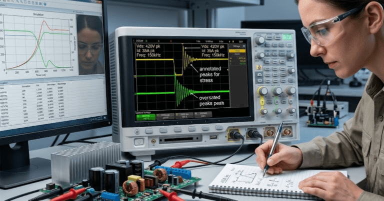
PHIL works for inverter testing only when the power interface preserves the electrical behaviour you are trying to study. The simulator computes the network response, the amplifier applies that response to the inverter terminals, and measured inverter output returns to the simulator. If that loop distorts timing or scaling, your result won’t represent the intended test case.
A three-phase grid-tied inverter is a good example. The simulated side contains the feeder impedance, utility source, and fault scenarios. The physical inverter sees commanded phase voltages at its AC terminals, then sends current back into the loop through sensors and the amplifier. If the bench has excess delay, the inverter can appear less stable than it really is. If the amplifier bandwidth is too low, harmonic behaviour can look cleaner than it should.
That is why interface quality decides test credibility before script details matter. Voltage range, current slew capability, measurement accuracy, scaling factors, and interface algorithm choice will shape what the inverter is allowed to show you. Good PHIL work makes those limits visible before anyone trusts the waveform plots.
Grid-connected equipment needs tight loop stability margins
Grid-connected PHIL setups work only when loop delay, source impedance, and interface dynamics stay inside stable margins. The physical unit, amplifier, sensors, and simulator form one closed electrical loop. If that loop is poorly tuned, a stable product can look unstable, or an unstable product can look acceptable for the wrong reason.
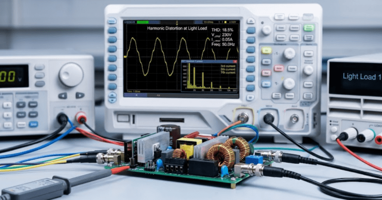
Weak-grid studies make this plain. A solar inverter tested against a simulated feeder with high impedance will react strongly to small phase and magnitude errors in the interface. A battery inverter under fault ride-through testing will also expose trouble quickly if current saturation in the amplifier is ignored. Utility-scale solar and battery storage were expected to account for 81% of new U.S. generating capacity additions in 2024. That mix puts far more grid equipment into cases where interface quality matters.
You will usually stabilize the setup with conservative test limits first, then widen the operating range once measured response matches your offline expectations. The safe order is impedance review, delay estimate, low-power shakedown, and only then full-stress cases. Skipping that order creates confusion that looks like product failure.
Your simulation model must respect bandwidth limits
A PHIL-ready simulation model keeps the physics that matter to the test objective and removes detail that the closed loop cannot support. You are preparing a model for a bandwidth-limited interface, with only the detail the setup can reproduce. If the model asks the bench to reproduce dynamics it cannot track, the test loses meaning.
A switching model of a 20 kHz inverter can behave well offline but overload a PHIL setup once amplifier delay and measurement filtering enter the loop. Teams often replace semiconductor-level switching with an averaged bridge model, while keeping the control delay, PLL response, current limits, filter resonance, and grid impedance that will affect the test outcome. That reduction keeps the important behaviour and drops detail the bench cannot honour.
Teams using SPS SOFTWARE for transparent offline modelling often catch missing delays, incorrect base values, or hidden parameter assumptions before moving the model into a PHIL workflow. That preparation matters because model reduction is not simplification for its own sake. It is disciplined selection of the dynamics the bench can represent honestly.
Unstable coupling can make good hardware look wrong
Bad PHIL coupling creates false failures because the bench can inject its own oscillations, phase error, clipping, and noise into the measured response. When that happens, you are testing the interface as much as the hardware. Good hardware will appear defective if the loop is poorly conditioned during closed-loop power exchange.
A converter that trips on overcurrent during PHIL does not always have a control problem. Sensor polarity errors, mismatched scaling, amplifier saturation, and hidden transport delay can all produce the same symptom. Another common trap appears when a device passes a nominal operating point but fails during a voltage sag, simply because the interface algorithm becomes unstable near that corner.
You can separate bench trouble from product trouble with a disciplined check sequence. Start with passivity and delay checks, compare measured small-signal response against the offline model, then repeat the case at reduced power. If the oscillation disappears only when the interface is softened, the setup is the first suspect. That mindset will save you from chasing faults that do not belong to the product.
“You are no longer checking code alone. You are checking how hardware behaves when the electrical system pushes back under load.”
PHIL pays off after software tests stop reducing uncertainty
PHIL pays off when controller HIL and offline simulation have already answered the software questions, but hardware-side uncertainty still blocks release, commissioning, or lab signoff. That is the point where more software study adds little value. The next useful step is to expose the physical unit to the electrical conditions that will decide acceptance.
That judgment keeps projects honest. A small educational inverter lab, an early control prototype, or a stable low-risk feeder study will often get enough confidence from offline modelling and controller HIL alone. A grid-tied converter facing weak-grid operation, strict fault response, and protection interaction usually will not. The difference is not budget theatre. The difference is the amount of unknown behaviour still sitting in the power path.
SPS SOFTWARE fits earlier in that chain, where you inspect equations, reduce models carefully, and enter PHIL with a test target you can explain line by line. Teams that treat PHIL as a late-stage proof tool, rather than a substitute for basic modelling discipline, will get cleaner failures, faster fixes, and results they can defend.