

Key Takeaways
- Capacitor bank switching overvoltage is set by the first milliseconds of the close, so time-domain study is required.
- Back to back bank arrangements and breaker behaviour often create the highest stress cases in a switching study.
- Mitigation only counts when waveform checks show lower peaks at every bus that hosts sensitive loads.
Capacitor bank switching must be studied as a transient event, because a routine close can create overvoltage that reaches far beyond the switched bus.
Steady-state reactive power checks won’t show the first peak, the inrush path, or the way nearby banks reflect the event back into the feeder. A Lawrence Berkeley National Laboratory study estimated that power disturbances cost U.S. businesses $104 billion to $164 billion each year, which gives short switching events practical weight beyond the waveform screen.
Capacitor bank energization creates steep transient overvoltage
Closing a capacitor bank connects an uncharged element to a live network, so the first milliseconds are set by the voltage difference, source inductance, and breaker timing.
“Steady-state reactive power calculations won’t reveal it.”
A 13.8 kV industrial bus can look calm in load flow, yet the same bus can ring sharply when a 2.4 Mvar bank closes near a lightly damped source. Sensitive power supplies respond to the peak rather than the reactive support. The ITIC voltage tolerance curve places 120% of nominal voltage outside the normal operating region once it lasts more than 0.5 cycle, which shows why a brief rise still matters when it reaches control circuits or drive front ends.
You need capacitor bank switching transient simulation because the damaging part of the event happens before the bank settles to its new steady voltage. Cable length, transformer leakage, and local load impedance all shape that first oscillation. If you only inspect the bus after the breaker is fully closed, you’ll miss the event that trips equipment.
Back-to-back banks magnify the first peak
Back-to-back switching is severe because an energized bank will discharge into the newly closed bank through very low inductance. That local exchange creates higher inrush current, higher frequency oscillation, and stronger voltage magnification than a single isolated bank energization case.
A common plant arrangement makes this easy to miss. One bank is already on the bus, a second bank closes for added reactive support, and the current path between them is only the short buswork and breaker connection. That path has little resistance, so the first current crest rises fast. Protection that never reacts to a remote feeder fault can still see sharp current spikes during this close.
Voltage magnification also appears away from the switched bus. A nearby motor control centre, a long cable to a variable speed drive, or a tertiary winding on a transformer can show a larger crest than the capacitor terminals themselves. That is why a capacitor bank switching study has to include adjacent buses and connected equipment, not only the bank that is being energized.
EMT simulation captures capacitor switching transients in time
EMT simulation captures capacitor switching transients because it resolves the waveform sample by sample through the switching instant. You can see the first peak, the oscillation frequency, the decay rate, and the way reflections move through feeders, transformers, and nearby capacitor banks.
A practical case study starts with the pre-switch steady state, then closes the breaker at defined angles across several runs. You’ll usually record bus voltage, capacitor current, breaker current, and the voltage seen by nearby loads. A 60 Hz phasor study cannot show the difference between a mild ring and a steep surge at a drive bus, but an EMT run will show it clearly.
That time view also helps you separate causes. One case might be dominated by local bus inductance, while another is set by a long cable reflection or a transformer capacitance path. When you model capacitor bank energization this way, mitigation moves from guesswork to direct comparison of waveforms, current peaks, and damping time.
A useful EMT model starts with stray inductance
Useful capacitor switching modelling starts with the inductance and resistance that sit between the source, breaker, bus, and capacitor bank. Those small elements set the inrush frequency and peak current, so an ideal source tied to an ideal capacitor will give a neat waveform that is physically wrong.
A short section of bus duct, a few metres of cable, or a small current-limiting reactor can change the shape of the event more than a large shift in steady-state load. A transparent model in SPS SOFTWARE lets you inspect those paths directly, which matters when you are checking why two similar banks produce very different switching records on site.
| Model element | Why it changes the switching waveform |
| Source Thevenin inductance and resistance | This branch sets how much current the upstream system can force into the bank during the first oscillation. |
| Bus duct and short cable sections | These small lengths often control the local oscillation frequency when banks sit close to the breaker. |
| Capacitor bank internal arrangement | Series and parallel groupings shift effective capacitance and can change the local current split during energization. |
| Current limiting reactor placement | Reactor location changes both the first peak and the damping seen at nearby buses. |
| Connected transformers and motor loads | These devices create alternate paths for reflected energy and can raise stress away from the switched bus. |
That level of detail does not make the study complicated for its own sake. It makes the result believable. You’re not trying to build every screw and bracket, but you’re trying to capture the electrical path that will shape the transient overvoltage and the inrush current seen by the breaker.
Breaker closing angle controls the worst energization case

Breaker closing angle matters because the voltage difference across the contacts at the instant of conduction sets the first charging surge. The worst case appears when the trapped capacitor voltage and source voltage create the largest mismatch at contact touch or prestrike.
A three-phase bank closing near a source voltage crest will not produce the same stress as a close near a zero crossing. Phase spread makes this more severe, because poles do not close at the exact same microsecond. One feeder can show a modest phase A peak and a much larger phase C peak simply because the pole timing and trapped charge line up badly.
You should treat closing angle as a sweep, not as a single run. A useful set of cases includes several point-on-wave positions and trapped voltage states after previous de-energization. That approach will show the true upper bound of the event, which is the value that matters when you are checking insulation margins and load ride-through.
Switch models must represent prestrike restrike behaviour
Switch models must represent prestrike and restrike because real interrupters do not always move from open to fully closed in one ideal step. Contact approach, dielectric breakdown, and current interruption can create extra voltage steps that raise stress above the clean close shown by an ideal switch.
Vacuum and air interrupters can show very different signatures during capacitor switching. A bank that looks acceptable with an ideal breaker can produce a harsher waveform once prestrike is added, because the capacitor starts to charge before mechanical contact seals. Another case can show restrike during opening, which means the study should not stop at energization if field records show complaints during both close and trip operations.
This matters most when you are testing protection pickups, surge arrester duty, or insulation coordination margins. An ideal switch is still useful for screening, but final settings and final mitigation checks need the switch behaviour that matches the breaker technology installed in the yard.
Mitigation should be tested at every affected bus
Mitigation works only when it reduces the crest and ringing at the buses that actually host sensitive equipment. A fix that looks good at the capacitor terminals can still leave a higher peak at a drive bus, transformer tertiary, or remote control panel.
A typical industrial feeder shows this clearly. A reactor at the bank may cut local inrush current well, yet a long cable to a process line can still see reflected overvoltage if the switching sequence is poor. You should test each measure at all affected observation points, then compare the worst remaining crest, oscillation frequency, and decay.
- Current limiting reactors reduce peak inrush current and shift the oscillation to a lower frequency.
- Controlled closing narrows the range of breaker angles that produce the highest stress.
- Switching order matters when one energized bank can feed the next close through a short bus path.
- Surge arresters should be checked at the buses where reflected peaks actually appear.
- Damping elements must be sized from waveform results rather than from steady-state ratings alone.
That process answers the common question of how to reduce switching overvoltage with evidence instead of habit. You’re checking the full surge path from source to affected bus.
Study results should guide switching timing policy
A capacitor bank switching study earns its value when results become operating rules for timing, sequencing, and permitted system states.
“Good policy comes from the worst verified waveform, the buses that saw the highest stress, and the mitigation that held those values inside acceptable limits.”
One utility feeder may need a rule that blocks a second bank close until the first bank is settled and a reactor is in service. Another plant may need a fixed sequence that keeps a long cable bus off line during capacitor energization. Those rules are simple, but they only stay credible when they come from waveform evidence instead of a generic switching note.
That is where a disciplined model pays off. SPS SOFTWARE fits this work because you can trace the physical path of the transient, inspect the assumptions, and turn a capacitor bank switching study into a clear operating practice that keeps routine switching from becoming a recurring source of trips.