

Free Trial
Free Trial
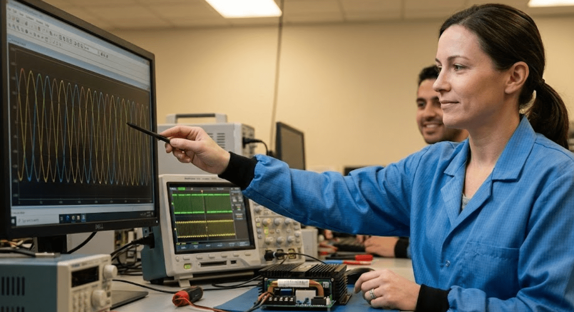
Engineer inspecting a power electronics board at a test bench
Modelling

Building high confidence MOSFET models from manufacturer datasheets

Key Takeaways

  • A reliable MOSFET model starts with the converter stress case, not the headline values in the datasheet table.
  • Conduction, charge, and capacitance fitting should be handled in sequence so each parameter set keeps a clear physical role.
  • Trust comes from validation against the original test conditions and from clear limits on where the model has been checked.

A MOSFET model built straight from headline datasheet numbers will miss the losses and waveforms that matter in converter simulation.

Electric motor systems use about 45% of global electricity, which means converter errors don’t stay small once they reach long duty cycles and high power ratings. You need a MOSFET model that reflects the test conditions behind each published curve, not just a few catalogue values. That is the difference between a simulation that only looks plausible and one that supports thermal, efficiency, and control work. High confidence comes from disciplined fitting, not from copying a default MOSFET spice model and hoping the datasheet agrees.

A good workflow starts with the converter stress you need to study, then fits conduction and switching behaviour as separate problems. You’ll get better results when you treat charge and capacitance as voltage-dependent effects and validate against the same tests used in the MOSFET datasheet. That approach gives you a model you can trust inside its calibrated range and question outside it.

Datasheet models fail when test conditions stay hidden

A datasheet curve only describes a MOSFET under the exact bench setup used to measure it. Gate resistance, drain voltage, junction temperature, and stray inductance all shape the published result. Hidden conditions turn copied values into wrong waveforms, even when the MOSFET datasheet looks complete and the model parameters seem reasonable.

A switching plot is a good example. A turn-on time measured at 400 V, 20 A, and 10 Ω gate resistance will not match a converter leg running the same device at 250 V with a 2.2 Ω gate resistor. The curve still has value, but only after you tie it to the stated test circuit. Footnotes, axis labels, and small captions often carry more modelling value than the headline part table.

You’ll also see hidden assumptions around temperature and package parasitics. A transfer curve taken at 25°C can fit threshold behaviour well and still miss current at 125°C. A vendor model that follows one output curve can still fail on turn-off overshoot because the test fixture inductance was never represented. Reading a MOSFET datasheet for simulation means treating every published plot as a conditional result, not a universal truth.

Start with the converter stress that sets accuracy needs

The right MOSFET model starts with the stress case that matters most in your converter. Voltage swing, current level, switching speed, and junction temperature decide which datasheet curves deserve the most fitting effort. A synchronous buck and a hard-switched boost converter will punish different modelling errors.

A 48 V to 12 V synchronous buck usually needs tight low-voltage conduction fitting, because a few milliohms of error will shift efficiency and heat rise at full load. A 400 V boost stage needs stronger charge and capacitance fitting, because switching loss and node overshoot will dominate. Power electronics process more than 70% of the electricity generated in the United States, so model accuracy matters most where converters spend their time and losses.

  • Match bus voltage to the highest and lowest values the device will actually see.
  • Match current to the operating band that sets your thermal limit.
  • Match junction temperature to the condition used for design review.
  • Match gate resistance to the driver network in your schematic.
  • Match switching frequency to the loss mechanism you need to predict.

This priority list keeps the work focused.

“You’re not trying to make a universal MOSFET model on day one.”

You’re trying to build a model that stays faithful where your converter lives. Once that operating window is fixed, parameter choices stop feeling arbitrary and start serving a defined simulation goal.

Separate conduction fitting from switching fitting early

Conduction fitting and switching fitting should be treated as two linked but separate tasks. Channel parameters control current and on-state drop, while charge and capacitance terms control transition timing and energy. Mixing both problems too early makes it hard to see which parameter caused the mismatch.

Start with the steady-state side. Fit the on-state slope and threshold region using output curves, transfer curves, and on-resistance data at the target temperature. A low-voltage server supply gives a clear case, because the simulated drain current at 4.5 V gate drive must line up before you touch rise and fall time. That first pass sets the channel behaviour without the noise of switching parasitics.

Move to switching only after the conduction fit is stable. A common failure shows up when someone stretches gate charge values to force a better turn-on delay, then wonders why the DC current no longer matches the datasheet. You’ll save time if each parameter set has one main job. That separation also makes later validation easier, because each error points to a smaller part of the model.

Use output curves to lock in channel behaviour

Use output curves to lock in channel behaviour

Output curves are the most direct path to a trustworthy channel fit. They show how drain current responds to drain-source voltage across several gate voltages, which lets you set threshold, transconductance, and on-state slope with much less guessing. A good fit here will stabilize every later step.

Pick the gate voltages that overlap your use case instead of fitting every curve with equal weight. A 10 V gate-drive industrial inverter cares far more about the high-current region than the sub-threshold knee. A 4.5 V logic-level design cares about the opposite. The model should match the slope near the operating current, the saturation bend, and the low-voltage resistive region at the same time.

Temperature data matters here too. If the datasheet gives on-resistance against temperature, use it to scale channel conduction after the 25°C fit is complete. That extra step stops the model from looking perfect on one bench plot and failing during thermal sweeps. The checkpoint below helps map the main datasheet plots to the fitting task they should control.

Datasheet plot What it should control in your model
Output characteristics Use these curves to set channel current response across the voltage and gate-drive range you actually switch.
Transfer characteristics Use this plot to refine threshold and transconductance where small gate-voltage errors create large current errors.
On-resistance against temperature Use this relation to keep conduction loss believable during thermal sweeps and hot-load checks.
Gate charge curve Use this plot to shape delay, Miller plateau behaviour, and the timing of voltage and current overlap.
Capacitance against drain voltage Use this relation to model non-linear switching, node ringing sensitivity, and output capacitance energy.
Reverse recovery test Use this test only if the body diode or commutation path matters in your converter leg.

Use charge curves to shape switching behaviour

Gate charge curves are the cleanest way to shape switching behaviour once the channel fit is stable. They capture how the gate current is spent across threshold, Miller plateau, and final enhancement. Rise and fall times only make sense after that charge partition lines up with the datasheet test.

A double-pulse style switching event shows why this matters. If the simulated Miller plateau is too short, drain voltage will collapse too quickly and turn-on loss will look falsely low. If total gate charge is correct but the split between pre-plateau and plateau charge is wrong, the waveform will still miss delay and overlap. You need the model to spend charge in the same order as the device.

Keep the gate loop explicit during this step. The driver voltage, external resistance, and source inductance all shape the current available to charge the gate. A model that matches a datasheet switching plot with the wrong gate network won’t travel well into your converter. This is where many generic MOSFET spice model files look convincing on paper and fail in a half-bridge simulation.

Treat capacitance plots as voltage-dependent functions

MOSFET capacitances are strongly non-linear, so fixed values will distort switching energy and waveform shape. Input, reverse transfer, and output capacitance should follow the drain voltage shown in the datasheet plots. A voltage-dependent fit is required if you want credible turn-off loss, ringing tendency, and dead-time behaviour.

A 400 V switching node makes this obvious. Output capacitance near 20 V can be several times larger than it is near 300 V, so a single Coss value will misstate both stored energy and drain-voltage slew. Reverse transfer capacitance also shifts the Miller effect as Vds changes. That means the same device can look tame in one operating region and much slower in another.

Piecewise fitting is often enough. You don’t need a perfect analytical expression if three or four voltage regions reproduce the plotted capacitance and stored-energy trend. Many engineers also forget the impact on soft-switching intervals and body-diode commutation. Once capacitance is treated as a function instead of a constant, the model starts to carry its weight in converter simulation.

Validate the model against the exact datasheet tests

Validation only means something when the simulation recreates the same test used in the MOSFET datasheet. Match bus voltage, load current, gate resistor, temperature, and reference points before judging the result. That discipline turns curve fitting into model verification instead of a visual comparison exercise.

A useful workflow is to rebuild the published switching or output-characteristic test bench first, then run the device model through the same conditions. If a turn-off plot was measured with a clamped inductive load, the simulation should use the same arrangement and probe points. SPS SOFTWARE fits well here because editable model structure makes it easier to trace a mismatch back to charge, capacitance, or parasitic assumptions instead of hiding it inside a closed block.

“Look for the shape of the error, not only the peak value.”

A correct current peak with the wrong plateau duration means one problem. A correct delay with too much overshoot means another. Validation becomes much faster once each mismatch is linked to a specific physical effect. You’ll also build a record of what the model has already passed, which matters when someone reuses it in another converter study.

Know where the model stops being trustworthy

A high-confidence model is only trustworthy inside the voltage, current, temperature, and gate-drive range used to calibrate it. Outside that range, the same model becomes an estimate. Good engineering practice means marking those limits clearly and refusing to treat one successful fit as universal proof.

A model tuned for a 100 kHz hard-switched leg at 25°C will not automatically predict behaviour in a 20 kHz motor drive at 125°C with a different gate network. The output curves, charge fit, and capacitance fit still provide a strong base, but trust comes from declared bounds. You should write those bounds into the model notes so the next user knows what has been checked and what has not.

That is the standard worth keeping. Converter studies rise or fall on the credibility of the device model inside them, and careful parameter work is what turns a MOSFET datasheet into something useful. SPS SOFTWARE supports that kind of work best when you need open, inspectable models that let you see why a waveform matches, why it misses, and where the model should stop speaking with confidence.


Modelling

Modeling renewable energy systems in electrical networks

Key Takeaways

  • Start with a single testable grid question, measured at the point of interconnection, with clear pass fail criteria that set model boundaries.
  • Pick EMT or RMS based on the grid phenomenon and time scale, then match inverter controls, limiters, and network strength to that purpose.
  • Validate every study against operating point, event timing, and impedance assumptions so plots translate into defensible engineering evidence.

Accurate renewable energy simulation depends on matching your model detail to the grid behaviour you need to prove.

Renewable plants interact with networks through controls, limits, and protection logic as much as through megawatts and megavars. Renewable power capacity additions hit 507 GW in 2023, which raises the stakes for studies that must be repeatable and defensible. Treat modelling as a scoped engineering test, not as a schematic drawing exercise.

You’ll get better results when you treat each simulation as a contract between inputs, assumptions, and outputs. That contract should say what grid event you care about, what you’re allowed to ignore, and what “correct” looks like. Once that is written down, choices like EMT versus RMS, inverter detail, and network equivalents stop being debates and start being traceable engineering selections. Teams that do this well spend less time rerunning studies and more time acting on results.

“Poor grid integration modelling usually fails for one reason: the study question is vague, so the model gets built with the wrong level of physics.”

Define the renewable system and grid question you must answer

A useful model starts with a single testable question and a clear point of interconnection definition. You should state the event, the metric, the pass fail threshold, and the required confidence level. You should also define what must be captured, such as unbalance, harmonics, or protection trips. Anything not tied to that question becomes optional detail.

Write down the modelling scope before you open a tool, because the scope sets your minimum model fidelity. Grid studies often mix concerns like fault ride through, flicker, voltage support, and protection coordination, but one model rarely answers all of those well at the same time. You’ll also need to set boundaries so the renewable plant model and the network model meet at the same electrical reference, with consistent base values, sign conventions, and measurement points. A good scope also states what you will treat as fixed, such as tap positions or capacitor states, and what you will vary across scenarios.

  • The point of interconnection location and the measured quantities at that bus
  • The grid event type and its timing including clearing and reclosing
  • The plant response metric such as voltage recovery time or current limit behaviour
  • The acceptance criteria tied to a grid code clause or internal requirement
  • The model exclusions that you will not interpret results against

Once the scope is fixed, you can make deliberate tradeoffs. If your question is about voltage recovery, inverter current limiting and network impedance matter more than energy yield. If your question is about feeder thermal loading, steady state power flow detail matters more than switching transients. You’re not trying to model everything; you’re trying to model the smallest set of physics that still forces the correct answer.

Choose EMT or RMS simulation based on grid phenomena

The main difference between EMT and RMS simulation is time scale and what electrical detail gets preserved. EMT keeps instantaneous waveforms, so it captures switching, unbalance, fast controls, and protection interactions. RMS keeps the slower phasor behaviour, so it captures voltage, frequency, and control responses without waveform detail. Your choice should follow the phenomenon, not the plant size.

RMS is the right starting point for many grid planning questions because it runs faster and supports large networks. EMT becomes necessary when the study involves fast inverter control loops, weak grid coupling, converter current limiting during faults, or interactions that depend on waveform shape. Hybrid workflows can also work, but they only help if the handoff between models is consistent and you keep the acceptance criteria tied to the original study question. SPS SOFTWARE users often treat this step as a modelling gate, because it prevents overbuilding EMT models for problems that RMS can answer cleanly.

What you need to learnSimulation type that fitsWhy the fit is strong
Voltage and frequency response over secondsRMSPhasor dynamics capture slower controls without waveform cost
Fault ride through current limits and fast control transitionsEMTInstantaneous modelling captures protection timing and current clipping
Unbalance and negative sequence effects at the point of interconnectionEMTPhase detail is preserved, so sequence coupling is explicit
Large area transfer studies with many buses and contingenciesRMSComputation stays manageable for wide network coverage
Switching transients and breaker or reclosing timing sensitivityEMTWaveform detail captures transient overvoltages and timing dependencies

Set numerical expectations early so the simulation stays stable and interpretable. EMT models need a time step small enough to resolve the fastest dynamics you included, and that usually means your inverter and network detail must be consistent with that step. RMS studies need careful selection of control time constants and measurement filters so the plant does not react faster than the model is able to represent. Good practice is to justify the method with a short statement tied to the event and the metric, then keep that statement attached to every result you share.

Model inverter controls, limits, and protection functions accurately

Renewables interact with power grids through control loops and limiters more than through static P and Q setpoints. You should model the control structure that actually drives current injection during disturbances, including measurement filters, phase tracking, and current references. You should also include limiters, rate limits, and priority logic, because those determine what the inverter can deliver under stress. Omitting these details makes fault and recovery results unreliable.

Start by identifying the inverter operating mode that matters for your study. Grid following controls rely on phase tracking and current regulation, so weak grids and faults can expose phase lock behaviour and current saturation. Grid forming controls set voltage and frequency references, so they require careful treatment of virtual impedance and power control to avoid nonphysical oscillations. In both cases, the limiter behaviour matters more than the small signal tuning when you’re evaluating ride through, because limiters decide when the control law stops being linear.

Protection modelling also needs discipline, because protection blocks often contain the trip logic that creates the outcome you’re trying to assess. Include undervoltage and overvoltage functions, frequency protection, and any fault ride through blocking logic that changes current injection commands. Use parameters from documentation or test reports, then sanity check them against the plant ratings and the grid code requirements that apply at the point of interconnection. If you cannot justify a parameter, mark it as an assumption and test sensitivity around it rather than hiding it inside the model.

Represent the network with feeders, transformers, and weak grid effects

Grid integration modelling fails when the network seen by the renewable plant is simplified past the point where it drives the wrong currents and voltages. You should represent the impedance and strength at the point of interconnection, plus the transformer and feeder elements that shape fault levels and voltage recovery. You should also preserve grounding and unbalance features if your acceptance criteria depends on them. Network fidelity should follow the disturbance path, not the geographic map.

Weak grid behaviour shows up when the Thevenin impedance is large compared to the plant rating, so small current changes cause large voltage swings. That affects phase tracking, voltage control, and protection thresholds, so the short circuit strength and X over R ratio are not optional details. Wind and solar generated 13.4% of global electricity in 2023, and that higher inverter share makes grid strength assumptions more visible in study outcomes. Transformer taps, leakage, saturation assumptions, and line charging also shape recovery behaviour, especially when reactive power control is active.

Network equivalents can be appropriate, but only if you preserve the features that matter to the plant response. A static Thevenin source can be enough for some fault ride through checks, while other studies need explicit upstream protection, load models, or generator dynamics. Keep base values consistent, check per unit conversions, and verify that the pre disturbance power flow and voltage profile match what you intended. When the network model is correct, odd inverter behaviour often becomes understandable instead of mysterious.

 “Good modelling judgment shows up when you can explain why a result is correct, not just show a plot that looks smooth.”

Set study scenarios for faults, switching, and grid code tests

Study scenarios should be built as controlled tests that isolate the grid phenomena you care about. You should define the disturbance waveform, the clearing sequence, and the pre-fault operating point, then run only the cases needed to cover your acceptance criteria. Faults, switching, and grid code tests are valuable because they force inverter limiters and protection logic to act. Clear scenario definitions also make results repeatable across tools and teams.

A concrete setup keeps this disciplined. A 100 MW solar plant connected through a 115 kV transformer to a long radial feeder with low short circuit strength can be tested with a three-phase fault at the point of interconnection, cleared after a specified time, then followed by an automatic reclose after a dead time. The key outputs would be terminal voltage recovery, reactive current injection behaviour during the fault, and any control mode transitions during the reclose. That single sequence will show you if the model captures current limiting, phase tracking stability, and protection blocking correctly.

Grid code style tests should be expressed as measurable requirements, not as vague expectations. Tie each case to a pass fail metric such as voltage recovery within a time window, reactive current response versus voltage deviation, or frequency support within a droop band. Keep initial conditions consistent, because small differences in reactive power, tap position, or controller state can change the response more than the disturbance itself. When you need many scenarios, group them by the physics they stress so you can trace failures back to modelling choices instead of guessing.

Validate results and avoid common renewable integration modelling errors

Validation is the step that turns simulation output into engineering evidence. You should confirm that steady state power flow, fault levels, and control limits match the plant ratings and the network assumptions. You should also check that events occur exactly when intended and that measurements are taken at the correct buses. Without these checks, even a sophisticated EMT model will produce confident-looking but wrong answers.

Most errors come from a few avoidable patterns. Initial conditions that do not match the intended operating point will distort controller behaviour and trip thresholds. Over-simplified limiters can produce nonphysical current injection that looks helpful during faults but cannot happen in hardware. Network impedance mistakes, especially base value and transformer impedance handling, often shift short circuit strength enough to flip a pass into a fail. Sensitivity checks should focus on the assumptions you marked earlier, since those are the ones most likely to control the outcome.

Good modelling judgment shows up when you can explain why a result is correct, not just show a plot that looks smooth. Keep model parameters transparent, keep acceptance criteria tied to the study question, and keep scenario definitions consistent, then results become easier to defend in reviews. SPS SOFTWARE fits well when you need physics-based, editable models that you can inspect line by line, because transparency forces the validation habits that keep studies honest. That discipline will matter more than any single tool setting, since long-term confidence comes from repeatable modelling practice, not from perfect looking waveforms.

Modelling

Why Interoperability Matters In Physical System Modelling

Key Takeaways

  • Interoperability matters because it keeps model intent stable as work moves across toolchains.
  • Data alignment and disciplined system exchange keep parameters, units, and results reproducible across teams.
  • Workflow clarity through ownership, versioning, and interface checks reduces rework and late-stage failures.

Physical system modelling breaks down when model intent, data, and interfaces shift as work moves across tools and groups. Interoperability matters because it keeps the meaning of your model stable as it’s edited, exchanged, and verified, so results stay traceable and engineering decisions stay defensible. A cost analysis of interoperability gaps estimated about $15.8 billion per year in avoidable costs for the U.S. capital facilities industry.

Teams often treat interoperability as file conversion, but the bigger risk is semantic drift. Parameters get reinterpreted, units get assumed, signals get renamed, and “the same” subsystem starts behaving like a different one. Strong interoperability practices keep models understandable across toolchains and over time, with fewer surprises during commissioning, lab validation, and design reviews.

“Interoperability turns a model into an asset your whole team can trust.”

Interoperability in physical system modelling means consistent model intent

Interoperability means the model you hand off keeps the same intent when someone else runs it. Intent includes the physical scope, operating point, required fidelity, and stated assumptions. When intent is consistent, a model remains interpretable across toolchains, and results stay comparable across studies.

Start with an explicit model contract that lives with the model, not in someone’s head. That contract states what the model represents, what it omits, and what “correct” looks like in terms of outputs and limits. It also defines sign conventions, reference directions, and initial conditions so downstream users don’t silently reverse meaning. Model intent also needs a clear boundary between physics and control so interface signals stay stable.

Intent discipline reduces debates that waste cycles in reviews, because reviewers can check purpose and assumptions before arguing about waveforms. It also stops well-meaning edits from turning one study model into a different study model under the same file name. When model intent is stable, the remaining interoperability work becomes mechanical rather than interpretive.

Toolchain compatibility reduces rework when models move between teams

Toolchain compatibility matters because most modelling work is collaborative and staged, not done in one tool by one person. When models move cleanly across toolchains, teams spend time improving physics and controls instead of rebuilding blocks, retesting, and revalidating results that already existed in another format.

Compatibility starts with choosing representations that survive exchange, like clear component boundaries, explicit interfaces, and parameter sets that don’t depend on hidden tool defaults. File formats matter, but compatibility also covers solver assumptions, initialization rules, and how events are handled. A model that relies on undocumented default tolerances will behave differently after exchange, even if the topology looks identical.

Tradeoffs are real. The most portable representation can limit access to tool-specific features, while a tool-optimized model can lock you into one workflow. Good teams separate “study models” from “implementation models,” then agree on where fidelity must match and where it can differ, so compatibility work stays focused on the parts that affect results.

Data alignment keeps parameters, units, and signals consistent everywhere

Data alignment keeps the numbers in your model from changing meaning when they cross a boundary. Units, scaling, naming, and signal definitions need to be consistent across tools, spreadsheets, scripts, and reports. When alignment is weak, teams can get the “right” plots for the wrong reasons, then discover the mismatch late.

A clear illustration is how unit handling can decide outcomes even when equations are correct. A unit mismatch contributed to the loss of a $125 million spacecraft, after one system produced values in imperial units while another assumed metric. Modelling teams face the same class of failure when a parameter table uses one base unit set and the simulation assumes another.

Alignment improves workflows when you treat data as a product with validation rules. Unit metadata should be attached to parameters and signals, not implied. Names should be stable and descriptive, and scaling should be explicit at interfaces so values don’t get “fixed” with hidden gains. Once data alignment is consistent, debugging shifts from chasing conversions to checking actual system behaviour.

System exchange needs common interfaces for models, results, and metadata

System exchange works when you share more than a model file. Teams need a common package that includes the model, its parameter sets, run configuration, and the minimum metadata required to reproduce results. Without that package, exchanges turn into “it runs on my machine” arguments.

Define what gets exchanged at each handoff and keep it consistent. The exchange package should include interface definitions, parameter dictionaries, unit annotations, initialization settings, and a small set of expected outputs used as acceptance checks. Results matter too: a baseline run with logged signals helps the receiving team confirm they’re running the same system, not a lookalike.

Execution improves when the exchange format matches how people actually review work. SPS SOFTWARE users, for instance, tend to benefit from exchange packages that keep component equations inspectable and parameter values traceable, because reviewers can verify intent without guessing what’s inside a closed block. That same idea applies in any toolchain: shared artefacts should support inspection, reproduction, and controlled change.

What you standardize for exchangeWhat stays consistent after a handoff
Interface signals with names, units, and sign conventionsTeams interpret inputs and outputs the same way across tools.
Parameter sets stored as versioned dictionariesRuns stay reproducible even after tuning and refactoring.
Initialization rules and operating pointsStart-up behaviour matches, so early transients remain comparable.
Run configuration including solver assumptions and tolerancesNumerical differences don’t get mistaken for physics differences.
Baseline results with agreed acceptance signalsRecipients can confirm equivalence before adding new work.
Metadata stating scope, omissions, and validity limitsModels don’t get reused outside the conditions they were built for.

Workflow clarity comes from explicit ownership, versions, and handoffs

Workflow clarity prevents interoperability work from turning into personal knowledge. Clear ownership, versioning rules, and handoff points make it obvious who can change what, when changes are reviewed, and how a model gets promoted from draft to trusted. That clarity is what keeps multi-team modelling from fragmenting.

Make handoffs explicit and lightweight, then treat them as part of engineering practice. Ownership should cover both model structure and data tables, since either can break a study. Version identifiers should link model changes to study outcomes, so a surprising result can be traced back to a specific edit. Handoffs should include a short acceptance check so the receiver confirms equivalence before building on top.

  • Assign one owner for interfaces and one owner for parameter data.
  • Tag every shared model with a version and a short change note.
  • Use a fixed handoff checklist that includes units and sign checks.
  • Store baseline run outputs with the model, not in personal folders.
  • Require review before interface signals or parameter names change.

These rules reduce rework because they shrink the space where silent changes can hide. They also make collaboration safer for students and new engineers, since expectations are written down. Clear workflows won’t remove technical disagreements, but they will keep disagreements focused on engineering rather than archaeology.

Checks that prevent failures when linking physics and control models

Linking physics and control models fails in predictable ways, and a small set of checks prevents most of them. The goal is consistency across domains, not perfect modelling. Interface checks, unit checks, and regression checks catch mismatches early, before teams spend weeks tuning a controller against a miswired plant model.

Start with interface checks that treat every boundary as a contract. Inputs and outputs should have expected ranges, units, and steady-state values under a known operating point. Add regression checks that rerun a small baseline case after any structural change and compare key signals within agreed tolerances. Include numerical sanity checks too, since step size, event handling, and initialization can change stability and damping without any physics change.

“Interoperability is not a separate workstream from model quality; it is model quality.”

Teams that practise disciplined checks get faster agreement, clearer reviews, and fewer late-stage surprises when work leaves the original author’s toolchain. SPS SOFTWARE fits well when you want transparent, inspectable models to support those checks, because inspection reduces guesswork and helps teams converge on shared understanding.

Modelling

How Open Modelling Environments Improve Integration Workflows

Key Takeaways

  • Open architecture keeps system models inspectable and editable, so integration effort shifts from file conversion to controlled interface work.
  • Interoperable workflows cut rework when interface contracts, versioning, and repeatable tests are treated as non-negotiable engineering practices.
  • Model exchange protects system intent only when units, assumptions, limits, and validation checks travel with the model across teams and tools.

Open modelling platforms improve integration workflows by keeping models portable and inspectable.

Integration work fails when models become trapped inside one tool’s file format, naming rules, and hidden defaults. Teams then spend time rebuilding the same logic in parallel, arguing about mismatched results, and rechecking assumptions that should have travelled with the model. Interoperability gaps can carry a measurable cost; inadequate interoperability in U.S. capital facilities was estimated at $15.8 billion per year. That number is not about simulation alone, but it matches the same pattern of avoidable translation and rework.

“Open architecture in modelling tools works because it shifts integration from one-off conversions to a repeatable workflow built on clear interfaces, transparent model definitions, and disciplined change control.”

Interoperable workflows will reduce rework only when your team treats model exchange as an engineering deliverable, not a last-minute export step. Integration flexibility is less about having more connectors and more about keeping intent intact as models move between people, stages, and tools.

Define open architecture in modelling tools for integration work

An open architecture modelling tool exposes the structure of a model, not just its outputs. You can inspect equations, parameters, and interfaces without guessing what the tool is doing behind the scenes. The model can be extended without rewriting it from scratch. Integration work becomes a controlled interface problem instead of a reverse-engineering exercise.

Open architecture usually shows up as readable model definitions, stable interfaces for connecting components, and a predictable way to package a model so another toolchain can consume it. You can trace where a parameter is set, see which units it assumes, and review how signals flow between subsystems. That transparency matters for technical leaders because it supports review, audit, and repeatable handoffs, even when different teams own different parts of the system.

Open architecture is also a constraint, and that’s a good thing. It forces agreement on what counts as the model boundary, which parameters are public, and which behaviours are guaranteed. Teams that skip this discipline still end up with “open” models that no one trusts, because each handoff changes behaviour in small, hard-to-detect ways.

Map common integration workflow bottlenecks that closed tools create

Closed tools slow integration because they hide assumptions and make model reuse depend on manual steps. You can run a simulation, but you cannot always verify how the tool interpreted your data or stitched blocks together. Export paths tend to drop metadata, rename signals, or flatten structure. Each handoff then turns into a fresh validation cycle.

Most bottlenecks are not technical limits of simulation, they are workflow limits. A closed format can prevent meaningful code review of model changes, since diffs are unreadable or meaningless. Automated testing becomes harder because model construction depends on interactive steps. Even a small interface change can force downstream teams to rebuild wrappers, re-map signals, and re-baseline results.

Closed tools also create organizational friction. Ownership becomes unclear when only a few specialists can open or modify the model. That pushes integration decisions later than they should happen, when schedule pressure is highest and mistakes are most expensive to fix. The result is a workflow that rewards local progress while penalizing system integration.

Interoperable workflows reduce rework across teams and toolchains

Interoperable workflows reduce rework because they standardize how models connect, how parameters are passed, and how changes are tracked. Teams can divide work without duplicating the same subsystem in multiple formats. Interface contracts make dependencies visible early. Integration flexibility then comes from consistent handoffs, not from heroics at the end.

A grid integration program often splits responsibilities between a network study team and a converter controls team. One group needs a stable representation of converter behaviour for system studies, while the other iterates on control logic and limits. A workable interoperable flow packages the converter model with a clear interface, version tag, and parameter set, so the network model can be updated without rewriting the converter block each time.

That approach improves more than speed. It improves accountability because each change can be traced to a model version and interface change, which makes review meetings shorter and technical disagreements easier to resolve. It also raises the bar for quality, since the cost of rerunning integration tests drops when model exchange is routine rather than exceptional.

Model exchange preserves system intent across simulation and design

Model exchange matters because a model is more than equations, it is intent captured as assumptions, limits, and interfaces. Intent gets lost when a model is reimplemented, simplified, or translated without a clear mapping of parameters and signals. That alignment is what prevents integration from turning into a debate about whose results are “right.”

Errors from miscommunication are not a small problem. Software errors were estimated to cost the U.S. economy $59.5 billion annually. Model exchange is one of the practical ways to reduce that class of error in engineering programs, since a consistent interface and shared assumptions cut the chance that two teams implement the “same” logic differently.

Good model exchange also supports governance. You can attach interface documentation, units, parameter ranges, and validation status to the exchanged model, so downstream users do not improvise. The tradeoff is that teams must accept stricter rules around interfaces and naming, because flexibility without constraints just moves confusion downstream.

“Preserving intent keeps teams aligned on what the model represents and what it deliberately ignores.”

Criteria to assess integration flexibility before standardizing on tools

Integration flexibility can be evaluated with a few practical checks that expose how a tool behaves under change. The key question is how much of your workflow can be automated and reviewed outside the tool’s user interface. You should also test how well intent survives a handoff to another team. If the integration path depends on manual “cleanup,” it will fail under schedule pressure.

  • Models remain readable and reviewable after export, not flattened into opaque artifacts.
  • Interfaces have explicit definitions for signals, units, and parameter ownership.
  • Model packaging supports versioning so changes can be tracked and rolled back.
  • Automation hooks exist for builds and tests so integration is repeatable.
  • Licensing and access rules do not block downstream teams from inspecting models.
What you need to integrateWhat breaks in closed toolsWhat open architecture should provide
You need an engineering review of model changes before merging.Binary or opaque files prevent meaningful diffs and approvals.Model definitions stay inspectable so reviews focus on behaviour changes.
You need consistent interfaces across multiple subsystems.Hidden defaults and implicit units cause mismatched results after handoff.Interfaces carry explicit units, ranges, and ownership expectations.
You need repeatable integration tests across model versions.Manual export and interactive setup makes tests non-repeatable.Packaging supports automation so testing is part of routine integration.
You need to swap subsystem implementations without rewriting the system model.Tight coupling forces rewiring and revalidation for every subsystem change.Stable boundaries let subsystems change while system connections remain intact.
You need cross-team access to inspect and adapt component models.Access limits create specialist bottlenecks and slow integration cycles.Editable models let more of the team contribute without guessing behaviour.

Tool choice still depends on your technical constraints, but the evaluation should be run like an integration rehearsal, not a feature checklist. Teams using SPS SOFTWARE often treat openness as a workflow requirement, since editable component models and transparent equations make interface discussions concrete instead of speculative. That focus keeps integration from becoming a late-stage scramble to reconcile mismatched assumptions.

Common interoperability failure modes and practical ways to prevent them

Interoperability fails in predictable ways, and most of them are avoidable. Unit mismatches, interface drift, hidden parameter defaults, and inconsistent initial conditions will break trust in exchanged models. Teams then “fix” issues locally, which silently forks behaviour across toolchains. Prevention depends on interface discipline and validation routines that run every time a model changes.

Start with strict interface contracts that define signals, units, and acceptable ranges, then treat any interface change as a breaking change that triggers review. Add lightweight validation models that check basic invariants like sign conventions, steady-state points, and saturation behaviour, so integration errors show up early. Version tagging needs to be mandatory, since “latest” is not a version, and untracked changes will always resurface during troubleshooting.

Interoperability also needs ownership. Someone must own the interface, not just the model internals, and that ownership must include documentation updates when behaviour changes. Teams that build these habits will get lasting integration flexibility from open architecture, because model exchange becomes predictable and testable. SPS SOFTWARE fits well when you want that discipline to be practical day to day, since transparent models make it easier to see what changed and why, which is what keeps integration work from repeating itself.

Modelling

Practical guide to modelling power converters and inverters

Key Takeaways

  • Start with a clear study question and set model fidelity only where it changes the outcome, since extra detail in the wrong place will slow simulation without improving trust.
  • Keep physics, controls, and numerics consistent across the full chain from device parasitics to PWM timing to EMT time step, because small mismatches will distort harmonics, losses, and fault response.
  • Use validation as a gate, not a formality, with checks that separate electrical behaviour, control timing, and solver sensitivity so results stay stable across operating points and disturbances.

Accurate power converter and inverter models come from disciplined modelling choices.

Converter results go off the rails when fidelity, solver settings, and control timing do not match the question you need answered. Grid studies now lean heavily on inverter behaviour, and renewables supplied 30% of global electricity generation in 2023. That scale leaves little room for hand waving around switching, limits, and protection response.

“Accurate power electronics modelling is less about adding detail everywhere and more about placing detail where it changes the outcome.”

You will get better confidence when you treat converter modelling as a chain of choices that must stay consistent from devices to controls to electromagnetic transient simulation time steps. The sections below focus on those choices, the tradeoffs they create, and the checks that prevent false certainty.

Define modelling goals and required fidelity for converter studies

Start by locking down the study outcome, then set the minimum model detail needed to answer it. Converter modelling always trades speed for waveform detail, and the wrong trade creates convincing but wrong results. Fidelity must match the phenomena that matters, such as harmonics, protection triggers, or control stability. A clear goal also sets the acceptable time horizon and solver time step.

Good goal setting also forces boundary decisions that quietly dominate results, such as what sits outside the converter model and what is pulled inside it. Draw a line around what you will trust as a fixed network and what you will treat as a controlled power electronic system. Make the acceptance criteria explicit early, since you will use it later during validation and tuning.

  • What measurable output will you trust, such as current ripple or voltage sag depth
  • Which frequencies must be correct, from fundamental to switching sidebands
  • Which events must be correct, such as faults, limit hits, and restarts
  • What time window must be covered, from milliseconds to seconds
  • What accuracy check will decide pass or fail against a benchmark

Choose switching averaged or hybrid converter model structures

Switching, averaged, and hybrid structures each answer different questions, and none is universally best. Switching models resolve commutation and PWM ripple but cost time step and runtime. Averaged models preserve control dynamics and power flow while discarding switching detail. Hybrid approaches keep switching where events matter and smooth the rest.

Pick the structure by asking which mechanism changes the decision you need to make. Harmonic compliance, dead time distortion, and semiconductor stress need switching detail. Controller tuning, weak grid stability, and active power setpoint response often fit averaged models if you represent limits and delays faithfully.

Study focusModel structure that fitsMain tradeoff you accept
Control loop tuning checksAveraged converter with limitsSwitching ripple is removed
Protection and fault clearingHybrid with switching near eventsMore setup and calibration work
Harmonics and dv or dt stressFull switching with parasiticsSmall time step and long runtimes
Energy yield and thermal trendsAveraged with loss modelsFast transients are simplified
EMI filter interactionsSwitching with detailed passivesParameter sensitivity increases

Hybrid models only help when the handoff is clean. Keep state variables consistent and avoid hidden filters that shift phase, since that will mask instability and distort converter behaviour.

Build device and passive component models with correct parasitics

Device models and passive parasitics control switching loss, ringing, and harmonic content, so idealized parts will mislead you. Semiconductor on state voltage, reverse recovery, and nonlinear capacitances alter current and voltage edges. Inductor and capacitor ESR and ESL shift damping and resonance. Parasitics must also match the physical layout scale you intend to represent.

Start with the simplest non ideal set that changes your answer, then add detail only when the acceptance check fails. Snubbers, DC link capacitance, and stray inductance often dominate dv or dt and overshoot, so they deserve attention even when the control model is perfect. Thermal coupling can stay outside the EMT model for many studies, but you still need a loss representation that is consistent with your switching waveforms.

Parameter quality matters more than parameter count. Treat vendor curves, lab measurements, and extracted parasitics as data you version and review, not as values you type once and forget, since small errors in capacitance or stray inductance can shift resonance enough to change protection triggers.

Represent PWM modulation and dead time in inverter simulation

PWM and dead time decide the waveform your network actually sees, so modelling them carelessly will flatten harmonics and hide distortion. Carrier based modulation and space vector modulation differ in switching patterns and harmonic distribution. Dead time changes the effective phase voltage based on current direction, and that creates low order distortion. Modelling also must match sampling, update rate, and gate timing assumptions.

Consider a two level three phase inverter with an 800 V dc link, 10 kHz PWM, and a 3 microsecond dead time feeding an L filter and a stiff 400 V line to line grid. A switching model that includes dead time and current polarity logic will show a clear shift in the fundamental voltage and added low order harmonics, while an ideal switch model will not. That difference will also shift current controller effort and can change limit hits during voltage sags.

Dead time compensation belongs in the control model if the physical controller uses it. Keep the gate commands aligned to the simulator time step so dead time is not quantized into something much larger than intended, since that will create distortion that looks like a hardware issue when it is only a modelling artefact.

Implement control loops and digital delays for stable results

Control modelling must include sampling, computation delay, and saturation behaviour, since those features set stability margins. A continuous controller dropped into an EMT model without discretization will overestimate phase margin. Digital delay also interacts with the network impedance and can create oscillations that look like weak grid problems. Limits, anti-windup, and rate constraints shape fault response and recovery.

Start with a control timing budget that matches the intended platform. Represent sample and hold, PWM update timing, and any filtering used for measured voltage and current. Keep the controller time base consistent with the electrical time step so the loop does not see noisy derivatives or artificial phase lag.

Fault response deserves special care. Current limits, voltage ride through logic, and phase locked loop behaviour set the output during sags and phase jumps, so you will want those blocks to be explicit and inspectable rather than hidden inside black box elements.

Select EMT solver settings and time steps for converters

EMT simulation for converters lives or dies on solver stability, time step choice, and event handling. Switching edges, discontinuous conduction, and control updates introduce stiffness that can destabilize a loose solver. The time step must resolve the fastest event you care about, not the slowest behaviour you hope to study. Poor settings will quietly distort losses, harmonics, and peak currents.

Inverter simulation matters because inverter-based generation is no longer a niche case, and wind plus solar supplied 13.4% of global electricity in 2023. That level of penetration pushes planners and operators to trust EMT results during faults, energization, and control interactions. Solver choices become part of the engineering outcome, not just a numerical detail.

Pick a fixed step only if it resolves switching and control timing without excessive runtime. Variable step methods can work for averaged models, yet they still need guardrails around discontinuities and limit blocks so the solver does not step over the event that matters.

Set initial conditions and operating points to reduce transients

Initial conditions decide whether the first cycles of your simulation are physics or startup noise. A converter starting with empty DC link capacitors and zero controller integrators will create large artificial transients. A good operating point sets voltages, currents, and controller states close to steady operation before events occur. That keeps analysis focused on the disturbance you care about.

Use a staged startup that matches the intended sequence, such as network energization, DC link charge, phase lock, and current loop closure. If the study is a fault, start from a solved steady state so the fault is the first major change. If the study is a setpoint change, ramp references smoothly to avoid step commands that a physical controller would never issue.

Controller initial states deserve the same attention as electrical states. Integrators, filters, and phase locked loop states should reflect steady measurements, or you will misread the settling behaviour as a tuning problem.

Validate models against measurements and known converter benchmarks

Validation is the step that turns a model into something you can trust for choices that carry risk. Compare against measurements when you have them, and against published benchmarks when you do not. Start with steady state power balance and fundamental phasors, then move to harmonics and transients. Each validation layer should reduce uncertainty, not just confirm what already looked right.

Separate validation targets into electrical, control, and numerical checks. Electrical checks include dc link ripple, filter resonance, and harmonic spectra at key operating points. Control checks include step response, limit behaviour, and recovery after disturbances. Numerical checks include time step sensitivity and consistency across solvers when the physics is unchanged.

Transparent, editable models make this work practical because you can trace an error to an equation or parameter instead of guessing. SPS SOFTWARE is often used in teaching labs and research teams for this reason, since the component equations and parameters stay visible for review and adjustment.

Fix common modelling mistakes that distort losses and harmonics

Most modelling failures come from a few repeatable mistakes, and fixing them is a discipline, not a last minute patch. Ideal switches hide loss and ringing. Missing parasitics shift resonances and can erase harmonic peaks. Misaligned control timing can create artificial stability that disappears on hardware, so the model must be audited like a design.

“Good converter modelling is a habit of consistency across layers, not a hunt for the fanciest block.”

Start with a short checklist and apply it every time the model changes. Confirm that the switching frequency, PWM update rate, and dead time align to the simulation time step. Check that passive values include ESR and ESL where resonance matters, and confirm that device loss calculations use the same waveforms you simulate. Run a time step sensitivity check so you know the waveform is not a numerical artifact.

Teams that treat models as inspectable engineering objects get repeatable outcomes and fewer late surprises, and SPS SOFTWARE fits naturally into that workflow when you need physics based transparency you can review and teach from.

1 2

Get started with SPS Software

Contact us
Cart Overview