

Key Takeaways
- Voltage stability analysis works best when you track reactive power margin, equipment limits, and control saturation instead of relying on voltage magnitude alone.
- PV curves, QV studies, and dynamic simulation answer different questions, so the right study sequence will save time and improve the quality of your engineering judgment.
- Protection coordination, feeder load behaviour, and inverter current limits will decide whether simulated margin is credible enough to support operating or planning choices.
Voltage stability analysis in simulation works when you treat reactive power margin as the main signal, not voltage magnitude alone.
Voltage collapse rarely starts as a single low-voltage reading. It starts when generators, capacitor banks, static compensators, or inverter controls run out of reactive support while transfer stress keeps rising. Wind and solar produced 13.4% of global electricity in 2023, which means more grids now depend on converter behaviour that must be represented properly in stability studies. Good voltage stability analysis will show you where the weak buses are, which limits bind first, and how protection will react when voltage recovery slows.
Useful simulation comes from disciplined model choices, not from a single study type. You’re trying to answer a practical engineering question about margin, collapse risk, or corrective action. That means your model will need credible load behaviour, realistic control limits, and a study method matched to the disturbance or loading pattern you care about. If those pieces are wrong, the plots will look clean and still tell you the wrong story.
“The key measure is reactive power margin.”
Voltage stability is about reactive power margin
Voltage stability is the ability of a power system to maintain acceptable voltage after load growth, switching, or a disturbance. The key measure is reactive power margin. A bus can sit near nominal voltage and still be close to collapse. That is why voltage magnitude alone won’t tell you enough.
Consider a transmission corridor feeding a heavy urban load pocket on a hot evening. Tap changers keep distribution voltage near target, induction motors draw more reactive current, and a nearby generator reaches its reactive limit. The voltage profile can still look acceptable for a short period, yet the system has almost no extra support left. A small line outage or another step in loading will push the bus toward the nose of the power-voltage curve.
This matters because voltage instability is usually a limit problem before it becomes a visible low-voltage problem. You need to track generator reactive ceilings, switched compensation steps, transformer tap action, and load sensitivity to voltage. If you don’t, you’ll confuse a healthy operating point with a fragile one. Good analysis starts with the question, “How much support is left before controls saturate?”
Start simulation with a credible network model
A credible network model includes the parameters and controls that actually shape voltage response under stress. You need correct line data, transformer taps, shunt devices, generator limits, load composition, and control logic. If any of those are simplified too far, the margin you calculate won’t match field behaviour.
A practical setup begins with a solved base case and a clear study boundary. A feeder study needs feeder regulators, capacitor switching logic, and motor-rich loads. A bulk system study needs generator excitation, reactive capability limits, and transfer paths that reflect the operating condition you’re testing. In SPS SOFTWARE, that execution step is useful because you can inspect and edit model equations and protection settings instead of accepting a closed result.
The fastest way to lose confidence in voltage stability analysis is to skip basic model checks. Use this minimum checklist before you start stressing the system.
- Confirm the base case power flow matches the intended operating condition.
- Check every reactive source for realistic limits and control priorities.
- Represent loads with voltage sensitivity that fits the study area.
- Verify transformer tap ranges, deadbands, and time delays.
- Include protection elements that will trip before collapse is complete.
Use PV curves to locate weak buses first
PV curve analysis is the quickest way to find where voltage stability margin is thin. You increase loading or transfer stress step by step and watch how bus voltage responds. The weak buses are the ones that approach the nose first. Those buses deserve your attention before deeper studies begin.
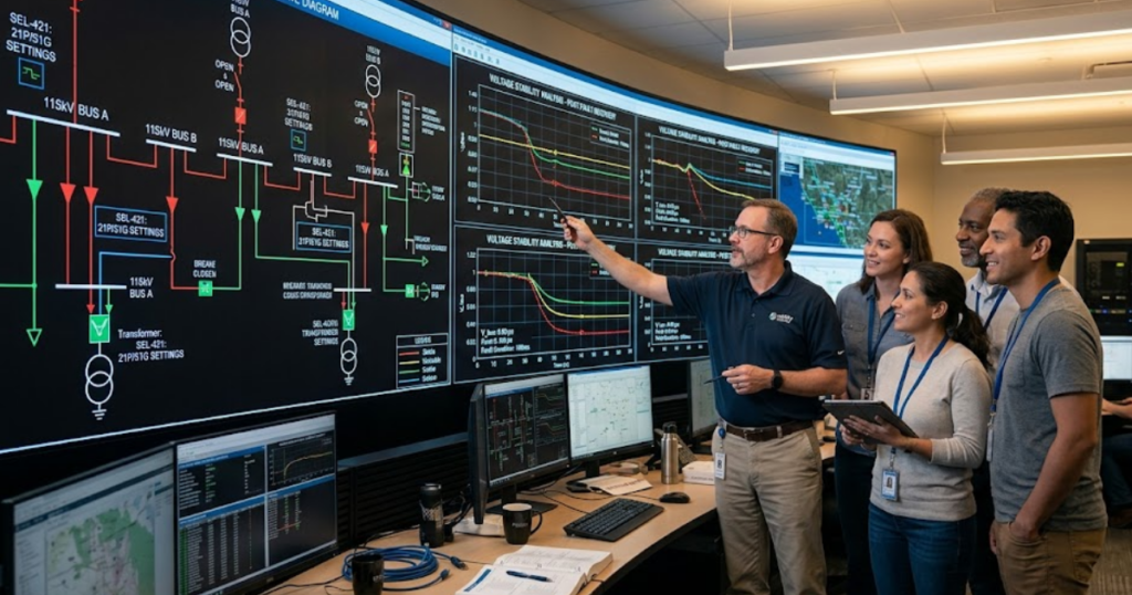
A common workflow stresses a transfer corridor from a generation area into a load area while monitoring several buses. One bus will usually show a sharper voltage drop and a smaller loadability margin than the others. That bus becomes the anchor point for corrective action screening. You can then test shunt support, generator redispatch, or tap adjustments and see which measure shifts the nose to a safer operating point.
PV curves are valuable because they turn a vague concern about collapse into a ranked map of weak locations. They also keep you from spreading effort across the whole network when the limiting problem is local. You’ll get the most value when each step respects equipment limits and control actions. If reactive ceilings are ignored, the curve will look better than the system really is.
Use QV studies when reactive limits dominate
QV studies answer a narrower but very important question. They show how much reactive injection a bus needs to maintain a chosen voltage level. That makes them useful when the main issue is local support deficiency. They are less about loadability and more about reactive deficiency at a specific location.
A weak substation bus near a large motor load is a good case. The PV curve can confirm that the area has poor margin, but the QV curve will show how much reactive support is required to hold 1.0 per unit or another target. That makes capacitor sizing, static compensation studies, and support placement more concrete. You’re no longer guessing which bus needs help or how much help it needs.
QV results become especially important after generator reactive limits are reached or after a line outage changes local VAR supply. They also expose cases where a bus needs support that a distant source can’t deliver effectively because of transmission reactance. If your question is “Where do I place support and how much is required?” a QV study will answer it more directly than a PV curve.
Dynamic simulation tests the path toward voltage collapse
Dynamic simulation shows how the system moves from a disturbance toward recovery or collapse over time. It captures control action, delay, saturation, and protection logic that static studies cannot represent fully. That is why it is essential after PV and QV studies identify weak areas. Static margin tells you the distance to trouble, while dynamic response shows the route.
A bus fault cleared after several cycles can leave motors stalled, transformer taps moving, and reactive devices switching in sequence. A static study will miss that timing. An RMS model can show slow voltage recovery after fault clearing, and a more detailed electromagnetic model can show converter current limiting or control interaction during the same event. Those details matter when the operating point is already close to its reactive ceiling.
Use this checkpoint to match the study method to the question you’re asking.
| Study approach | What it tells you clearly | When it is the best fit |
| Base case power flow review | It confirms that voltages, flows, and reactive outputs match the operating condition you intend to study. | Use it before any stability test so every later result starts from a credible state. |
| Power-voltage curve analysis | It ranks weak buses by showing where voltage collapses first as loading or transfer stress rises. | Use it when you need a quick view of margin and bus weakness across the network. |
| Reactive-voltage curve analysis | It shows how much local reactive support is required to hold a chosen voltage at a bus. | Use it when placement and sizing of var support are the main questions. |
| RMS disturbance simulation | It captures slower control action such as excitation, tap changes, motor recovery, and protection timing. | Use it after a fault, outage, or switching event when time response will shape the outcome. |
| Electromagnetic transient simulation | It resolves converter limits and short-term control interaction that are too detailed for steady-state methods. | Use it for inverter-rich areas or when switching and control detail will alter voltage recovery. |
| Protection coordination review | It shows which elements will trip first and how those trips alter the stability margin you thought you had. | Use it before final judgement so the simulated margin reflects the actual protection scheme. |
Distribution networks need load models that match behaviour
Distribution voltage stability studies will fail if load models are too simple. Feeders are shaped by motors, thermostatic loads, rooftop generation, regulator action, and unbalance. Constant power assumptions can overstate or understate collapse risk. You need behaviour that matches the actual feeder mix.
A long feeder serving air conditioning, small commercial motors, and distributed generation will respond very differently from a feeder made mostly of resistive heating. After a fault or voltage dip, motor stalling can hold reactive consumption high while regulators and capacitor controls respond with delay. If your model treats all of that as a static constant power block, the predicted recovery will look smoother than the feeder will actually deliver.
Distribution studies also need attention to where controls act and how quickly they act. Tap changers can support customer voltage while pushing the upstream system closer to its limit. Capacitor banks can help one section and worsen another if switching logic is poorly timed. You can’t study voltage collapse risk on a feeder as if it were a reduced bulk bus. The feeder’s composition is the study.
Grids with high renewable share need inverter limits
Renewable-heavy grids need explicit inverter current limits, control priorities, and reactive support settings in the model. Converter-based resources do not respond like synchronous machines. When voltage drops, their controls will follow current limits and protection thresholds. If those limits are missing, the simulated margin will be overstated.
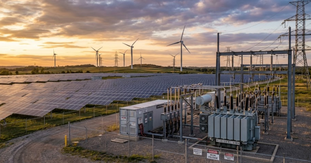
A solar plant tied to a weak grid offers a clear case. During a voltage dip, the inverter controller will often prioritise reactive current support up to a current ceiling. Past that ceiling, active power support falls and further voltage support is capped. Solar photovoltaic generation rose by almost 320 TWh in 2023, the largest annual increase ever recorded, which makes this modelling detail important for modern stability studies.
You’ll also need to represent plant-level voltage control, collector system impedance, and grid code settings that govern fault ride-through. A generic source behind a reactance won’t capture those limits. That shortcut might be acceptable for rough screening, but it won’t support a credible judgment about collapse risk. If your network is rich in inverter-based resources, the voltage stability model has to reflect converter physics and control logic.
“A margin that exists only before a relay trip is not usable margin.”
Protection coordination must reflect voltage stability limits
Power system protection coordination is part of voltage stability analysis because protection will define the final outcome once voltage recovery slows or current rises. A margin that exists only before a relay trip is not usable margin. You need the study to reflect the same trip logic the field equipment will enforce.
A delayed undervoltage trip on a wind plant, a load-shedding stage on a weak feeder, or an overexcitation limiter on a generator can each alter the path from disturbance to collapse. One setting can preserve service long enough for voltage recovery, while another can remove support and deepen the dip. That is why protection review belongs inside the simulation workflow instead of after it. If the relay clears first, your PV or QV result won’t be the whole answer.
The best engineering judgment comes from lining up margins, control limits, and protection timing in one consistent model. SPS SOFTWARE fits naturally in that workflow because open models make it easier to inspect the assumptions behind network response and relay action. You’re not looking for a dramatic plot. You’re looking for a study result that still makes sense when the system is stressed, the controls saturate, and the protection acts exactly as set.